
14.2: The Complexity of Genomic DNA
- Page ID
- 16500

By the 1960s, when Roy Britten and Eric Davidson were studying eukaryotic gene regulation, they knew that there was more than enough DNA to account for the genes needed to encode an organism. It was also likely that DNA was more structurally complex than originally thought. They knew that cesium chloride (CsCl) density gradient centrifugation separated molecules based on differences in density and that fragmented DNA would separate into a main and a minor band of different density in centrifuge tube. The minor band was dubbed satellite DNA, recalling the Sputnik satellite recently launched by Russia. DNA bands of different density could not exist if the proportions of A, G, T and C in DNA (already known to be species-specific) were the same throughout a genome. Instead, there must be regions of DNA that are richer in A-T than G-C pairs and vice versa. Analysis of satellite bands that moved further on the gradient (i.e., were more dense) than the main band were indeed richer in GC content. Those that lay above the main band were more AT-rich.
Consider early estimates of how many genes it might take to make a human, mouse, chicken or petunia: about 100,000! We know now that it takes fewer! Nevertheless, even with inflated estimates of the number of genes it takes to make a typical eukaryote, their genomes contain 100-1000 times more DNA than necessary to account for 100,000 genes. How then to explain this extra DNA? Britten and Davidson’s elegant renaturation kinetics experiments revealed some physical characteristics of genes and so-called ‘extra’ DNA. Let’s look at these experiments in some detail.
A. The Renaturation Kinetic Protocol
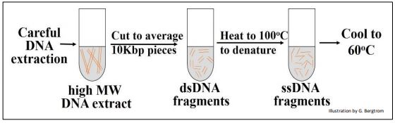
The first step in a renaturation kinetic experiment is to shear DNA isolates to an average size of 10 Kbp by pushing high molecular weight DNA through a hypodermic needle at constant pressure. The resulting double-stranded fragments (dsDNA) is then heated to 100oC to denature (separate) the two strands. The solutions are then cooled to 600C to allow the single stranded DNA (ssDNA) fragments to slowly re-form complementary double strands. At different times after incubation at 60oC, the partially renatured DNA was sampled and ssDNA and dsDNA were separated and quantified.
The experiment is summarized in the drawing below.
The amount, or percent of DNA that had renatured over time could be graphed.
B. Renaturation Kinetic Data
A plot of dsDNA formed at different times (out to many days!) is shown below for a renaturation kinetics experiment using rat DNA.
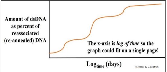
In this example, the DNA fragments could be placed in three main groups with different overall rates of renaturation. Britten and Davidson reasoned that the dsDNA that had formed most rapidly was composed of sequences that must be more highly repetitive than the rest of the DNA. The rat genome also had a lesser amount of more moderately repeated dsDNA fragments that took longer to anneal than the highly repetitive fraction, and even less of a very slowly re-annealing DNA fraction. The latter sequences were so rare in the extract that it could take days for them to re-form double strands, and were classified as non-repetitive, unique (or nearly unique) sequence DNA, as illustrated below.
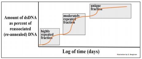
It became clear that the rat genome (in fact most eukaryotic genomes) consists of different classes of DNA that differ in their redundancy. From the graph, a surprisingly a large fraction of the genome was repetitive to a greater or lesser extent.
238 Discovery of Repetitive DNA
When renaturation kinetics were determined for E. coli DNA, only one ‘redundancy class’ of DNA was seen, as is shown below.
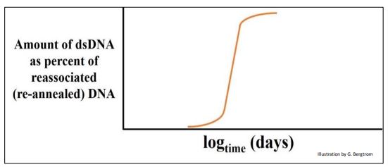
Based on E. coli gene mapping studies and the small size of the E. coli ‘chromosome’, the reasonable assumption was that there is little room for ‘extra’ DNA in a bacterial genome, and that the single class of DNA on this plot must be unique-sequence DNA.
C. Genomic Complexity
Britten and Davidson defined the relative amounts of repeated and unique (or singlecopy) DNA sequences in an organism’s genome as its genomic complexity. Thus, prokaryotic genomes have a lower genomic complexity than eukaryotes. Using the same data as is in the previous two graphs, Britten and Davidson demonstrated the difference between eukaryotic and prokaryotic genome complexity by a simple expedient. Instead of plotting the fraction of dsDNA formed vs. time of renaturation, they plotted the percent of re-associated DNA against the concentration of the renatured DNA multiplied by the time that DNA took to reanneal (the CoT value). When CoT values from rat and E. coli renaturation data are plotted on the same graph, you get the CoT curves in the graph below.
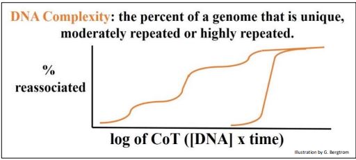
This deceptively simple extra calculation (from the same data!) allows comparison of the complexities of any number of genomes. These CoT curves tell us that ~100% of the bacterial genome consists of unique sequences, compared to the rat genome with its three DNA redundancy classes. Prokaryotic genomes are indeed largely composed of unique (non-repetitive) sequence DNA that must include single-copy genes (or operons) that encode proteins, ribosomal RNAs and transfer RNAs.
D. Functional Differences between CoT Classes of DNA
The next question of course was what kinds of sequences are repeated and which are ‘unique’ in eukaryotic DNA? Eukaryotic satellite DNAs, transposons and ribosomal RNA genes were early suspects. To begin to answer these questions, satellite DNA was isolated from the CsCl gradients, made radioactive and then heated to separate the DNA strands. In a separate renaturation kinetic experiment, rat DNA was sampled at different times. The isolated Cot fractions were once again denatured and mixed with heat-denatured radioactive satellite DNA. The mixture was then cooled to allow renaturation. The experimental protocol is illustrated below.
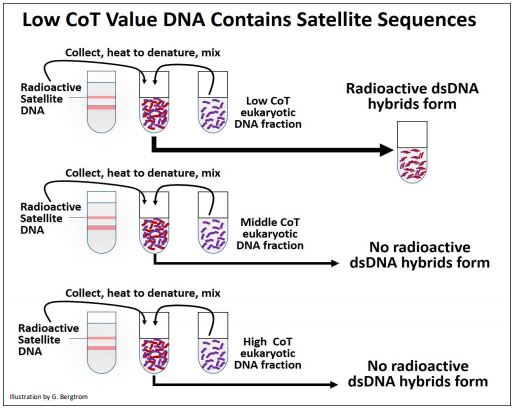
The results of this experiment showed that radioactive satellite DNA only annealed to DNA from the low Cot fraction (highly repeated) fraction of DNA. Satellite DNA is thus highly repeated in the eukaryotic genome. In similar experiments, isolated rRNAs made radioactive formed RNA-DNA hybrids when mixed and cooled with the denatured middle CoT fraction of eukaryotic DNA. Thus, rRNA genes were moderately repetitive. With the advent of recombinant DNA technologies, the redundancy of other kinds of DNA were explored using cloned genes (encoding rRNA, proteins, transposons and other sequences) to probe DNA fractions obtained from renaturation kinetics experiments. Results of such experiments are summarized in the table below.
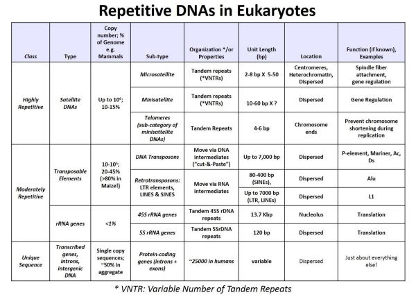
The table compares properties (lengths, copy number, functions, percent of the genome, location in the genome, etc.) of different kinds of repetitive sequence DNA. The observation that most of a eukaryotic genome is made up of repeated DNA, and that transposons can be as much as 80% of a genome was a surprise!
240 Identifying Different Kinds of DNA Each CoT Fraction
241 Some Repetitive DNA Functions
We’ll focus next on the different kinds of transposable elements