7.4: Modified Shoot
- Page ID
- 18021
Like leaves and roots, shoots and stems also have modifications. Some examples are rhizomes, stolons, tubers, bulbs, corms, thorns, spines, cladophylls, and stem traps. Rhizomes (example: ginger, Zingiber) are underground stems that burrow into the ground just below the soil surface, and usually tend to have small, scale-like leaves that are not photosynthetic. Buds from the axils of the leaves make new branches that will grow to become aboveground shoots.
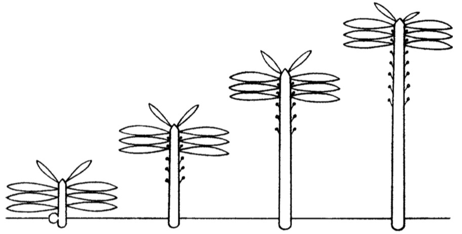
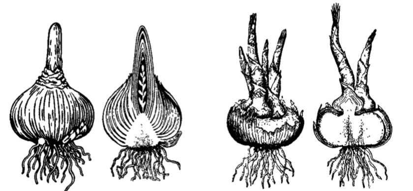
Stolons (runners) are aboveground horizontal shoots, which sprout and produce a new plants (example: strawberry, Fragaria). Tubers (example: potatoes, Solanum) are enlarged portions of rhizomes. The “eyes” of potato are actually lateral buds and the tuber body is comprised of many parenchyma cells that contain amyloplasts with starch. Corms and bulbs are shoot structures that are used for storage. A corm (example: crocus, Crocus) is a short, thick underground storage stem with thin scaly leaves. A bulb (example: onion, Allium) differs from a corm in the fact that it stores its nutrients in its fleshy leaves (Figure \(\PageIndex{2}\)).
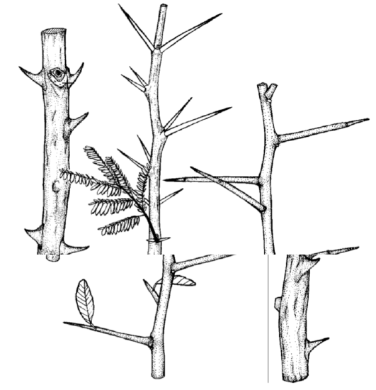
Thorns (example: hawthorn, Crataegus) are defensive shoots that help to protect the plant from predators. Spines are not modified stems, but rather modified, reduced leaves or stipules, or bud scales (example: almost all cacti, Cactaceae family). Prickles (example: rose, Rosa) are modified surface tissues of stem.
Cladophylls (examples: Christmas cactus, Schlumbergera; ribbon plant, Homalocladium) are leaf-like, flattened shoots. Phyllodes are actually leaf modifications (example: Australian acacias, Acacia) they visually similar to cladophylls but originated from flattened leaf petioles. Shoot insect traps are used by some carnivorous plants, such as bladderwort (Utricularia). The following table emphasizes the diversity of organ modifications:
| Leaf | Stem | shoot | |
|---|---|---|---|
| Absorption | Absorption leaves (bromeliads) | Rhizoids | Default |
| Defense | Spines, scales | Thorns, prickles | Spines |
| Expansion | Plantlets | Rhizomes, stolons, runners | Adventive buds |
| Interactions | Traps, sticky epidermis, urns, colored leaves | Traps, insect nests | Haustoria, mycorrhizae, root nodules, nematode traps, insect nests |
| Photosynthesis | Default, phyllodes | Cladophylls | Green roots (orchids) |
| Storage | Succulent leaves, pitchers | Bulbs, corms, tubers | Storage roots |
| Support | Tendrils, false stems, floats, suckers | Default, tendrils | Buttress, aerial and contractile roots, suckers |
Please note that superficially similar structures (e.g., shoot and leaf tendrils) might have different origin.
Raunkiaer’s Approach
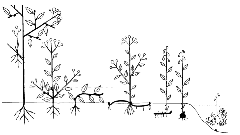
Christen Raunkiaer used a different approach to classify life forms which is useful to characterize the whole floras (all plant species growing on some territory), especially temperate floras. He broke plants down into six categories: epiphytes, phanerophytes, chamaephytes, hemicryptophytes, cryptophytes and therophytes.
Epiphytes do not touch soil (they are aerial plants), phanerophytes have their winter buds exposed, chamaephytes “put” their winter buds under the snow, winter buds of hemicryptophytes on the soil surface, cryptophytes in the soil and/or under water, and therophytes do not have winter buds, they go through winter as seeds or vegetative fragments (Figure \(\PageIndex{4}\)). Typically, northern floras have more plants of last categories whereas first categories will dominate southern floras. Note that Raunkiaer “bud exposure” is not far from the hardiness in the dynamic approach explained below.
Dynamic Approach
There are many life forms classifications. This is because life forms represent numerous secondary patterns in plan diversity, along with the main pattern which taxonomy wants to describe.
Dynamic life forms classification uses the fact that in nature, there are no strict borders between different life forms. If we supply the pole to some shrubs, they may start to climb and therefore become vines. In colder regions, trees frequently lose their trunks due to low temperatures and form multiple short-living trunks: they become shrubs. Conversely, in tropics, many plants which are herbs in temperate regions, will have time to develop secondary tissues and may even become tree-like.
Dynamic approach uses three categories: hardiness, woodiness, and slenderness (Figure \(\PageIndex{5}\)). Hardiness is a sensitivity of their exposed parts to all negative influences (cold, heat, pests etc.) This is reflected in the level of plant exposure, plants which are hardy will expose themselves much better. Woodiness is the ability to make dead tissues, both primary and secondary (reflected in the percentage of cells with secondary walls). High woodiness means that plants will be able to support themselves without problems. Slenderness is an ability to grow in length (reflected in the proportion of linear, longer than wide, stems). Low slenderness results in rosette-like plants. Combining these three categories in different proportions, one may receive all possible life forms of plants.
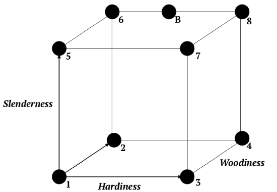
These three categories could be used as variables of the 3D morphospace. Every numbered corner in the morphospace diagram (Figure \(\PageIndex{5}\)) represents one extreme life form:
- Reduced floating annuals like duckweed (Lemna). Please note that zero hardiness is impossible; duckweed hardiness is just low.
- Short annual herbs like marigold (Tagetes); they accumulate wood if warm season is long enough.
- Bulb perennials like autumn crocus (Colchicum).
- Australian “grass trees” (Xanthorrhea) with almost no stem but long life.
- Herbaceous vines like hops (Humulus).
- Monocarpic tree-like plants like mezcal agave (Agave).
- Perennial ground-cover herbaceous plants like wild ginger (Asarum).
- Trees like redwood (Sequoia).
What is even more important, all possible positions on the “surface” and inside this cube also represent life forms. For example, the dot marked with “B” are slender, woody but only partly hardy plants. The partial hardiness means that vertical axes will frequently die, and then new slender woody axes develop from scratch. Woody wines and creeping bushes will correspond well with this description. As you see, this morphospace not only classifies existing plants but also could predict possible life forms.


