1.8: Serial Dilutions and Standard Curve

Learning Objectives

Goals:

• Prepare solutions starting with a solid.
• Perform a serial dilution.
• Use the spectrophotometer to measure the absorbance of solutions.
• Generate a standard curve and use the standard curve to determine the concentration of a solution.

Student Learning Outcomes:

Upon completion of this lab, students will be able to:

• Determine the mass of solute needed to make at %(w/v) solution.
• Make a buffer of the appropriate concentration.
• Make a stock solution of the appropriate concentration.
• Create a series of solutions of decreasing concentrations via serial dilutions.
• Use the spectrophotometer to measure the absorbance of a solution.
• Use excel and make a standard curve and use the R2 value to evaluate the quality of the standard curve.
• Use the standard curve to calculate the concentration of a solution.

Introduction

A Serial dilution is a series of dilutions, with the dilution factor staying the same for each step. The concentration factor is the initial volume divided by the final solution volume. The dilution factor is the inverse of the concentration factor. For example, if you take 1 part of a sample and add 9 parts of water (solvent), then you have made a 1:10 dilution; this has a concentration of 1/10th (0.1) of the original and a dilution factor of 10. These dilutions are often used to determine the approximate concentration of an enzyme (or molecule) to be quantified in an assay. Serial dilutions allow for small aliquots to be diluted instead of wasting large quantities of materials, are cost-effective, and are easy to prepare.

Equation 1.

\[concentration factor= \frac{volume_{initial}}{volume_{final}}\nonumber\]

\[dilution factor= \frac{1}{concentration factor}\nonumber\]

 

Figure 1. A ten-fold serial dilution, which can also be called a 1:10 dilution, or a series with dilution factor of 10. To determine the concentration at each step of the series, you divide the previous concentration by the dilution factor.
*Dilution tubes begin with 9-mL. 1-mL is added and mixed, then 1-mL is transferred to the next tube. The ending volume in the last tube would be 10-mL

 

Key considerations when making solutions:

• Make sure to always research the precautions to use when working with specific chemicals.
• Be sure you are using the right form of the chemical for the calculations. Some chemicals come as hydrates, meaning that those compounds contain chemically bound water. Others come as “anhydrous” which means that there is no bound water. Be sure to pay attention to which one you are using. For example, anhydrous CaCl₂ has a MW of 111.0 g, while the dehydrate form, CaCl₂ ● 2 H₂O has a MW of 147.0 grams (110.0 g + the weight of two waters, 18.0 grams each).
• Always use a graduate cylinder to measure out the amount of water for a solution, use the smallest size of graduated cylinder that will accommodate the entire solution. For example, if you need to make 50 mL of a solution, it is preferable to use a 50 mL graduate cylinder, but a 100 mL cylinder can be used if necessary.
• If using a magnetic stir bar, be sure that it is clean. Do not handle the magnetic stir bar with your bare hands. You may want to wash the stir bar with dishwashing detergent, followed by a complete rinse in deionized water to ensure that the stir bar is clean.
• For a 500 mL solution, start by dissolving the solids in about 400 mL deionized water (usually about 75% of the final volume) in a beaker that has a magnetic stir bar. Then transfer the solution to a 500 mL graduated cylinder and bring the volume to 500 mL
• The term “bring to volume” (btv) or “quantity sufficient” (qs) means adding water to a solution you are preparing until it reaches the desired total volume
• If you need to pH the solution, do so BEFORE you bring up the volume to the final volume. If the pH of the solution is lower than the desired pH, then a strong base (often NaOH) is added to raise the pH. If the pH is above the desired pH, then a strong acid (often HCl) is added to lower the pH. If your pH is very far from the desired pH, use higher molarity acids or base. Conversely, if you are close to the desired pH, use low molarity acids or bases (like 0.5M HCl). A demonstration will be shown in class for how to use and calibrate the pH meter.
• Label the bottle with the solution with the following information:
  • Your initials
  • The name of the solution (include concentrations)
  • The date of preparation
  • Storage temperature (if you know)
  • Label hazards (if there are any)

Lab Math: Making Percent Solutions

Equation 2.

Formula for weight percent (w/v):

\[ \dfrac{\text{Mass of solute (g)}}{\text{Volume of solution (mL)}} \times 100 \nonumber \]

Example

Make 500 mL of a 5% (w/v) sucrose solution, given dry sucrose.

1. Write a fraction for the concentration \[5\:\%\: ( \frac{w}{v} )\: =\: \dfrac{5\: g\: sucrose}{100\: mL\: solution} \nonumber\]
2. Set up a proportion \[\dfrac{5\: g\: sucrose}{100\: mL\: solution} \:=\: \dfrac{?\: g\: sucrose}{500\: mL\: solution} \nonumber\]
3. Solve for g sucrose \[\dfrac{5\: g\: sucrose}{100\: mL\: solution} \: \times \: 500 \: mL \: solution \: = \: 25 \: g \: sucrose \nonumber\]
4. Add 25-g dry NaCl into a 500 ml graduated cylinder with enough DI water to dissolve the NaCl, then transfer to a graduated cylinder and fill up to 500 mL total solution.

Activity 1: Calculating the Amount of Solute and Solvent

Calculate the amount (include units) of solute and solvent needed to make each solution.

A. Solutions with Soluble Solute and water as the solvent

1. How many grams of dry NaCl should be used to make 100 mL of 15% (W/V) NaCl solution?
2. How many grams of dry NaCl should be used to make 300 mL of 6% (W/V) NaCl solution?
3. How many grams of dry NaCl should be used to make 2L of 12% (W/V) NaCl solution?
4. How many grams of dry NaCl should be used to make 300 mL of 25% (W/V) NaCl solution?
5. How many grams of dry NaCl should be used to make 250 mL of 14% (W/V) NaCl solution?

B. Solutions with Insoluble Solutes in Cold Water

1. Calculate how to prepare 200 mL 1.2% (w/v) agarose in 1X SB buffer, given dry agarose and SB buffer.
2. Calculate how to prepare 300 mL 2.5 % (w/v) agarose in 1X SB buffer, given dry agarose and SB buffer.
3. Calculate how to prepare 50 mL 1.5 % (w/v) agarose in 1X SB buffer, given dry agarose and SB buffer.
4. Calculate how to prepare 60 mL 0.8 % (w/v) agarose in 1X SB buffer, given dry agarose and SB buffer.
5. Calculate how to prepare 150 mL 1.8 % (w/v) agarose in 1X SB buffer, given dry agarose and SB buffer.

Note

For dry chemicals that cannot dissolve in cold water (such as agarose and gelatin), pour the dry solute directly into an Erlenmeyer flask, measure the total volume of solvent in a graduated cylinder, then add the total volume of solvent into flask. Microwave the solution as recommended until solute is dissolved.

Part I: Solution Prep of 30-mLs of 13.6% Sodium Acetate

Sodium Acetate Buffer solutions are inexpensive and ideal to practice your skills. Your accuracy can be verified by taking a pH reading.

MATERIALS

Reagents

• Sodium Acetate (Trihydrate) solid
• DI H2O
• Stock bottle of verified 1 Molar Acetic Acid solution

Equipment

• pH meter
• Stir plate
• Electronic balance and weigh boats
• 50-mL graduated cylinder
• 50-mL conical tubes (Falcon tubes)
• P-1000 Micropipettes with disposable tips (or 5 mL Serological pipettes with pumps)

Calculations

• Calculate the amount of sodium acetate needed to make 30 mL of 13.6% sodium acetate solution.

Procedure

1. Make sure to wear goggles and gloves.
2. Measure _______ g of solid sodium acetate in a weigh boat on an electronic balance.
3. Transfer the sodium acetate into a 50 mL conical tube.
4. Add about 20 mL of DI water into the conical tube.
5. Secure the cap on the tube and invert to mix the contents until the solute is completely dissolved.
6. Pour out all of the solution into a 50 mL graduated cylinder.
7. Add DI water to bring the total volume to 30.0 mL.
8. Transfer all of the solution back into your 50 mL conical tube and secure the cap.
9. Invert the tube several times to thoroughly mix the contents.
10. Label the tube with contents (13.6% Sodium Acetate), initial, and date.

Verify your work by creating a buffer solution

1. Pipette exactly 5.0 mL of your sodium acetate solution into a clean 15 mL conical tube (or 25 mL glass test tube).
2. Pipette exactly 5.0 mL of 1M acetic acid solution into your conical tube (or 25 mL glass test tube).
3. Secure the cap on the conical tube (or a piece of parafilm over the test tube opening).
4. Invert several times to thoroughly mix the 10 mL of solution into an acetate buffer.
5. Measure the pH of the test buffer solution using a calibrated pH meter.
6. If you were accurate in all of your work, the test buffer should have a pH of 4.75 (+/- 0.06).
7. Check in with your instructor and report the pH of your test buffer.
8. If your test buffer pH is within the expected range, then congratulations! You have verified that the sodium acetate solution you made earlier has a concentration of 13.6%. Give your 50 mL tube of remaining sodium acetate solution to your instructor to save for use in a future lab.
9. If your test buffer pH is far outside of the expected range then something went wrong during the preparation of your sodium acetate solution and you should mark the tube with an “X” and give it your instructor to set aside.

Part II: Preparation of a Standard Curve

In this part of the lab, we will be preparing solutions of known concentrations. These then will be used to create a standard curve. Standard curves (also known as calibration curves) represent the relationship between two quantities. The standard curve will be used in part 3 of the lab to determine the concentrations of unknown solutions of methylene blue.

Materials

Reagents

• Stock 1% (w/v) methylene blue solution – (500 microliter (µL) aliquots in 1.5 mL microcentrifuge tubes)
• DI H₂O

Equipment

• P-20 Micropipettes and disposable tips
• P-1000 Micropipettes and disposable tips
• Spectrophotometer

Glassware

• 10 mL serological pipettes and pumps
• 1.5 mL microcentrifuge tubes
• 15 mL plastic conical tubes with screw-top caps
• 50 mL plastic conical tubes with screw-top caps

Calculations

1. Calculate the volume of stock 1% methylene blue solution needed to make 40 mL of 0.0005 % methylene blue solution.
2. This new percentage concentration is equivalent to 5.0 micrograms per milliliter (µg/mL) and will be the concentration of our working solution for the next 2 parts of the lab exercise.

Procedure

Prepare Stock Solution of Methylene Blue

Prepare 40 mL of 5.0 µg/mL Methylene Blue Working Solution

1. Make sure to wear goggles and gloves.
2. Very accurately pipette 40.0 mL of DI water into a 50 mL conical tube.
3. Very accurately micropipette ________ µL of 1% stock methylene blue into the DI water in your tube.
4. Secure the cap on the tube and invert repeatedly to thoroughly mix the solution.
5. Label your tube as “5.0 µg/mL Methylene Blue”, your name, and date.

Prepare Known Concentrations of Methylene Blue Working Solution via Dilution

Prepare 80% Methylene Blue Working Solution

1. Pipette 8.0 mL of 5.0 µg/mL methylene blue working solution into a 15 mL conical tube.
2. Pipette 2.0 mL DI H2O into the tube to make 10.0 mL of total solution.
3. Seal the tube and invert repeatedly to mix.
4. What is the concentration of your new solution? Label the tube _______ µg/mL methylene blue.

Prepare 60% Methylene Blue Working Solution

1. Pipette 6.0 mL of 5.0 µg/mL methylene blue working solution into a 15 mL conical tube.
2. Pipette 4.0 mL DI H2O into the tube to make 10.0 mL of total solution.
3. Seal the tube and invert repeatedly to mix.
4. What is the concentration of your new solution? Label the tube _______ µg/mL methylene blue.

Prepare 40% Methylene Blue Working Solution

1. Pipette 4.0 mL of 5.0 µg/mL methylene blue working solution into a 15 mL conical tube.
2. Pipette 6.0 mL DI H2O into the tube to make 10.0 mL of total solution.
3. Seal the tube and invert repeatedly to mix.
4. What is the concentration of your new solution? Label the tube _______ µg/mL methylene blue.

Prepare 20% Methylene Blue Working Solution

1. Pipette 2.0 mL of 5.0 µg/mL methylene blue working solution into a 15 mL conical tube.
2. Pipette 8.0 mL DI H2O into the tube to make 10.0 mL of total solution.
3. Seal the tube and invert repeatedly to mix.
4. What is the concentration of your new solution? Label the tube _______ µg/mL methylene blue.

Measuring Absorbance of Methylene Blue Working Solutions

1. Turn on the spectrophotometer and let it warm up for at least 10 minutes.
2. Place 1 mL of DI water into a clean cuvette. This is your blank.
3. Place 1 mL of your methylene blue solutions into clean cuvettes. These are your samples.
4. Set the wavelength of the spectrophotometer to 664 nm.
5. Place the blank into the spectrophotometer.
6. Press the “Zero” button and wait for the Absorbance to read “0.00”
7. Take out the blank and set aside.
8. Place your first sample into spec and record the absorbance reading. Do not press any buttons.
9. Repeat with each sample and record into lab notebook

Results

Complete Data Table 1. based on your results. Put in your notebook

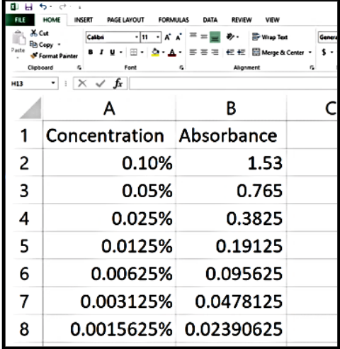
Figure 1. Completing the Excel table

Note this is an example: do not use these values for your concentration or absorbance

Table 1. Absorbances of Methylene Blue at Various Concentrations

Percentage of Working Solution Conc.	Methylene Blue Concentration (µg/mL)	Absorbance @ 664 nm
100%	5.0
80%
60%
40%
20%

Making a Standard Curve

1. Enter the data into Excel in adjacent columns.
2. Select the data values with your mouse. On the Insert tab, click on the Scatter icon and select Scatter with Straight Lines and Markers from its drop-down menu to generate the standard curve.

Figure 2. An example of a standard curve

1. To add a trendline to the graph, right-click on the standard curve line in the chart to display a pop-up menu of plot-related actions. Choose Add Trendline from this menu. Select “display equation on chart” and “display R-squared value on chart”. Ideally, the R2 value should be greater than 0.99.
2. Use the equation to determine the concentration of the sample solution by entering the absorbance for y and solving for x.
3. Print the standard curve and add to your notebook.

Part III: Determining Concentrations

Serial dilutions are quick way of making a set of solutions of decreasing concentrations. In this part of the lab we will make a series of dilutions starting with the Methylene Blue solution prepared in part 2 of this lab. Then, we will us the spectrophotometer to determine the absorbance of each solution. Once we know the absorbance, we will use the equation from your standard curve prepared in part 2, to determine the actual concentrations of each of your solutions.

Materials

Reagents

• 5.0 µg/mL Methylene Blue Working Solution
• DI H2O

Equipment

• P-20 Micropipettes and disposable tips
• P-1000 Micropipettes and disposable tips
• Spectrophotometer
• 5 mL serological pipettes and pumps
• 15 mL plastic conical tubes with screw-top caps

Preparation of Methylene Blue Solutions

Using the remainder of your 5.0 µg/mL methylene blue working solution from part 2, perform a set of 1:2 serial dilutions to make the following concentrations of the solution (50.0 %, 25.0 %, 12.5 %, 6.25 %, 3.125 %, and 1.5625 %).

Diagram of 1:2 Serial Dilutions

In your notebook, draw a diagram showing the serial dilutions for the 6 methylene blue solutions you are preparing. In the diagram, indicate the volume being withdrawn from the concentrated solution, the volume of water added, the concentration of the new solution, and the total volume.

Procedure

Preparation of Methylene Blue Concentrations via Serial Dilutions

Making 1:2 dilutions

• Pipette 5.0 mL of the 5.0 µg/mL methylene blue working solution into a 15 mL conical tube.
• Pipette 5.0 mL of DI water into the tube for a total of 10 mL of solution.
• Cap and mix well.
• Label this tube “50.0% MB”

Making 1:4 dilution

• Pipette 5.0 mL of the 50.0% MB solution into a new 15 mL conical tube.
• Pipette 5.0 mL of DI water into the tube for a total of 10 mL of solution.
• Cap and mix well.
• Label this tube “25.0% MB”

Making 1:8 dilution

• Pipette 5.0 mL of the 25.0% MB solution into a new 15 mL conical tube.
• Pipette 5.0 mL of DI water into the tube for a total of 10 mL of solution.
• Cap and mix well.
• Label this tube “12.5% MB”

Continue with this process to make the 1:16, 1:32, and 1:64 serial dilutions.

Write the procedures you used to make the solutions in your lab notebook.

Measuring absorbance

1. Follow the procedures in part 2 to prepare the spectrophotometer
2. Measure the absorbance values of the diluted solutions
3. Record the absorbance values and concentrations in your lab notebook in a table as shown below.

Data Table 2

Dilution Factor	% of Working Solution Concentration	Absorbance @ 664 nm	Methylene Blue Conc. (µg/mL)
1:2	50.0%
1:4	25.0%
1:8	12.5%
1:16	6.25%
1:32	3.125%
1:64	1.5625 %

Calculations

Use the equation from your standard curve in part 2 and the absorbance values of your solutions from Part 3, to determine the actual concentration of your solutions.

Study Questions

1. Describe how you would prepare 50.0-mL a 0.10% NaOH solution. In your description, include a calculation and step by step procedures including glassware.

2. It is common for solutions that are used often in a lab (or which are time consuming to prepare) to be intentionally prepared to be many times more concentrated than needed. For example, if a 1.36% sodium acetate is often used in the lab, then the 13.6% sodium acetate solution prepared in part 1 can be labeled as “10X” sodium acetate solution because the concentration is 10 times greater than needed. This way, you can save on storage space for the solution and you can quickly and easily dilute any desired amount of this to the correct concentration right before use.
3. Describe how you would prepare 100.0 mL of 10X sodium acetate solution. In your description, include a calculation and step by step procedures including glassware. Make sure to include steps to verify your solution by checking the pH.
4. Describe how you would prepare 100.0 mL of 1X sodium acetate solution from the 10x sodium acetate solution prepared in the questions above. In your description, include a calculation and step by step procedures including glassware.
5. Using a serial dilution, describe how you would prepare 10 mL of a 1%, 0.1% and 0.01% solution of NaOH. The stock solution of NaOH is 10%. Draw diagram as part of your description.
6. Using the standard curve below, calculate the concentration of an unknown solution if its absorbance is 0.55.

   

   Figure 3. A standard absorbance curve of Copper II

7. Evaluate the quality of the standard curve above by using the R2 value.