
32.01A: The Basics of Climate Change
- Page ID
- 97987

Search Fundamentals of Biochemistry
- to demonstrate how climate has changed over geological time through the present
- to explain mechanisms, using knowledge from biology, chemistry, and physics, for climate change
- to show the central role of atmospheric CO2 as a causative agent of past and present climate change
- to contrast the effects of anthropogenic burning of fossil fuels on climate change with causes of past climate changes
- to address arguments made by climate change skeptics
Introduction
We've known for a very long time that burning fossil fuels and releasing CO2 into the atmosphere would warm our climate. Perhaps the first paper addressing this, Circumstances affecting the Heat of the Sun's Rays, was published in 1856, before the US Civil War, by a woman scientist, Eunice Foote. John Tyndall (of the Tyndall effect) published more comprehensively on greenhouse gases in 1859. Given the complexity of the biosphere's climate, it was not until the 1980s that climate models became sophisticated enough for scientists like James Hansen to become convinced and alarmed enough to discuss in Congressional hearings the role of anthropogenic (made by humans) CO2 released into the atmosphere as a cause of ever-worsening global warming. The knowledge of human-induced climate change has been politicized and subjected to an orchestrated campaign of misinformation and disinformation by fossil fuel companies and their political contributors. We have delayed global actions for so long that we must act immediately and aggressively to address climate change before we reach climatic conditions that are so austere for humans that parts of the world become uninhabitable. Homo sapiens evolved in a world dominated by repetitive glaciation and deglaciation. Hans Joachim Schellnhuber, an atmospheric physicist, climatologist, and founding director of the Potsdam Institute for Climate Impact Research, has stated that humans have so affected the world that we have eliminated the possibility of the next glaciation cycle.
Many readers might not be familiar with the data and models supporting human-caused climate change and that climate scientists are almost unanimous in their support of the data and models. As in any field, however, you will find outliers who don't and whose ideas carry disproportionate weight among climate change skeptics. Hence, we provide the basic data to show the relationship between increasing atmospheric CO2 to global warming, both drought and flooding, ocean acidification, and loss of biodiversity. We also provide supportive information that would allow users to address questions from those who question the reality of present human-induced climate change. We don't shy away from using basic physics as well since most students studying biochemistry at the level found in this book have also studied physics as well as biology. In subsequent sections, we will then address the biochemistry of climate change and its mitigation.
Greenhouse Effect
Before the advent of the Industrial Revolution, the Earth's climate was fairly constant since the last ice age, which peaked about 22,000 years ago (YA) and ended about 12,000 YA. There have been short (on a geological time scale) periods of cooling since the end of the last ice age. Humans evolved around 200,000 years ago with modern civilizations arising about 4000 BCE so it could be said that humans are ice-age peoples (a distinctly Northern Hemisphere perspective). Humans have had the benefits of a fairly stable climate since then.
The sun's energy warms the Earth. If the Earth did not radiate back into space an equivalent amount of energy, it would slowly and continually warm. The Earth reflects energy back in the form of light. In addition, as the Earth is heated by the sun, the Earth releases heat in the form of infrared light (as do all warm objects). Earth's temperatures are stable when the sum of the energy emitted by the Earth equals the energy it receives from the sun. This is illustrated in Figure \(\PageIndex{1}\).

Figure \(\PageIndex{1}\): Energy balance for Earth as it adsorbs and emits solar radiation
Our stable climate has been enabled by fairly constant levels of atmospheric CO2, a trace atmospheric gas, which has hovered around 280 parts per million (ppm) until the start of the Industrial Revolution in 1770. CO2 is a greenhouse gas, which as anyone who has run an IR spectra knows, absorbs in the infrared. CO2 in the atmosphere absorbs some of the infrared radiation released by the Earth, allowing the Earth to be warmer than in its absence. The CO2 effectively acts as an insulating blanket. In fact, without CO2 or other "greenhouse" gases, the Earth would be completely covered by snow.
Other greenhouse gases in the atmosphere include methane and nitrous oxide. The IR spectra of these gases are shown in Figure \(\PageIndex{2}\). Students who have taken organic chemistry labs and obtained IR spectra of samples always blank the instrument to remove spectral signals from both CO2 and H2O.


Figure \(\PageIndex{2}\): IR spectra of some greenhouse gases. NIST (ex: https://webbook.nist.gov/cgi/cbook.c...ndex=1#IR-SPEC)
Since the start of the Industrial Revolution, humans have been releasing into the atmosphere ever-increasing amounts of CO2 from the burning of fossil fuels and methane from agricultural practices and natural gas production. CO2 levels, as of November 2022 have reached 415 ppm, while methane has increased to 1900 part per billion (ppb) or 1.9 ppm. Increasing methane in the atmosphere contributes about 20% of the global warming effect of the more concentrated CO2, given methane's intense IR absorbance spectra. It has a short half-life in the atmosphere (about 20 years) compared to that of CO2 (hundreds of years). Nitrous oxide (N2O) is also a powerful greenhouse gas, which also depletes ozone in the stratosphere. Our increased use of synthetic fertilizers and manure is the primary anthropogenic source of N2O. Its emission is accelerated from poorly drained farmlands.
The net effect is that the Earth is no longer in energy balance. The net contributions of energy input and output are expressed as energy/sec/m2 of the Earth's surface area. Hence the units are Joule/s.m2 = Watts/m2, where 1 Watt is 1 J/s. From around 2005 to 2019, the average Earth Energy Imbalance (EEI) (or budget) was about +460 x 1012 W or 460 terrawatts (TW) = 4.6 x 10¹⁴ W. Dividing this by the surface area of the planet (5.1 x 10¹⁴ m2), gives an average global value of +0.90 ± 0.15 W/m2 (or J/(m2s)). Newer and more refined estimates show it to be +1 W/m2 with most of the excess energy stored in the Earth's Oceans, which have a high specific heat capacity and cover 71% of the surface area of the planet. Most of the rest of the excess energy is used to warm land masses and melt ice shields and glaciers. 1 W/m2 might not seem like a lot but it is (pardon the pun), astronomically big.
The atomic bomb dropped on Hiroshima released about 1.8 x 10¹³ Joules (some estimates are as high as 9 x 10¹³ Joules) of energy. Assume for the sake of calculation that this energy was released in 1 second over the entire surface of the planet (5.1 x 10¹⁴ m2). The earth energy imbalance for that 1 explosion was 0.035 J/m2.s (0.176 J/m2.s for the higher estimate). The ratios of the present imbalance (+1 W/m2) to the distributed bomb's imbalances are 1/0.035 = 28x for the lower energy estimate bomb or 1/0.176 = 5.7 for the higher energy estimate. Hence the present imbalance, 1 J/m2s from human-caused climate change, is equivalent to detonating from 6-28 Hiroshima-type atomic bombs every second. Other estimates are lower and closer to 600 bombs per day but the bases for the calculation are not readily available. Regardless, these values should give you a dramatic sense of the imbalance and how unsustainable it is.
Figure \(\PageIndex{3}\) below shows a graphical representation of the Earth's energy budget.
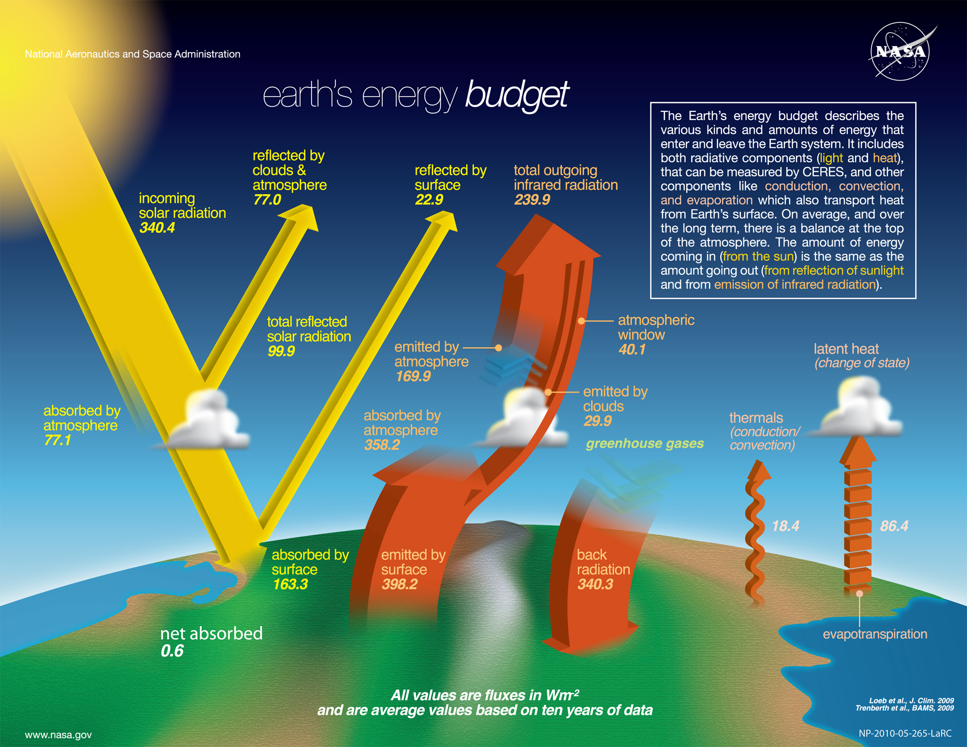
Figure \(\PageIndex{3}\): Earth's energy budget, with incoming and outgoing radiation (Values are shown in W/m2). Satellite instruments (CERES) measure the reflected solar and emitted infrared radiation fluxes. Year 2021 update: Net absorbed energy (shown as 0.6) rose to above 1.0 W/m2 based on independent CERES and ocean heat content measurements.(see fig.1 in Loeb et al.(2021), Geoph. Res. Let 48 (13), doi:10.1029/2021GL093047). Public Domain
The global warming potential (GWP) is used to calculate the total contribution of all emitted greenhouse gases. It is expressed in units of CO2 equivalents. It adds the contribution of other greenhouse gases like CH4 and nitrous oxide (N2O), each of which has unique IR absorption spectra (as shown in Figure 2 above) and atmospheric half-lives. The IPCC uses a 100-year time frame for the calculation of the GWP, which is often abbreviated as GWP100, and uses this formula:
\begin{equation}
\mathrm{CO}_2 \text { equivalent } \mathrm{kg}=\mathrm{CO}_2 \mathrm{~kg}+\left(\mathrm{CH}_4 \mathrm{~kg} \times 28\right)+\left(\mathrm{N}_2 \mathrm{O} k g \times 265\right)
\end{equation}
- CO2 has GWP of 1 by definition since it is the reference. Its time frame in the atmosphere (100s to 1000 years) doesn't matter since it is the reference.
- CH4 has a GWP of around 27-30 over 100 years. It reflects its higher IR absorbance but lower life-time (around 12 years).
- N2O has a GWP of around 265-273 over a 100-year timescale. N2O has a life-time of around 109 years.
Water is also a greenhouse gas as you can attest to on humid days and how its lack in the atmosphere in deserts leads to a large temperature drop at night. It's very different than other greenhouse gases. Its concentration varies enormously (from 40 ppm to 40000 or more) based on humidity and precipitation events, which remove it from the atmosphere. The amount of water in the atmosphere increases with increasing global temperatures, which gives rise to more intense precipitation events and also to warmer temperatures in a positive feedback loop. Its concentration in the atmosphere hence changes enormously on the time scale of hours and days, so its half-life in the atmosphere is short. In contrast, the half-life of CO2 in the atmosphere is measured in decades to centuries.
The basis for methane's contribution to climate change needs a clearer explanation. It is a very potent greenhouse gas, given its absorption spectra in the IR. Many oil companies have indicated a commitment to decrease the leakage of methane from pipelines, which would be helpful, but these efforts may draw attention away from the fact that CO2 is by far the biggest problem. Over 20 years (not 100 as in the GWP calculations above), methane is 80 times as potent as CO2. Those numbers sound ominous (80X and 20 years, which is not long away)! But you shouldn't compare the two on a kg/kg basis, as the warming from CO2 could last 1000 years but from methane only 20 years after which it disappears. The long-term climate effect for methane, given its short lifetime in the atmosphere, depends on the rate (megatons/year) it is added to the atmosphere, but for CO2 it is the net mass added over a longer time which has a cumulative effect. CO2 effects continue to increase, but methane effects wain quickly. So you can't easily compare warming over the first 20 years. Consequently, a delay in acting on methane is minimal compared to a delay in acting on CO2.
Methane contributes to about 30% of the net warming, and about 60% of the methane is probably from human activities. As we hit the IPPC Paris target of 1.5 0C, about 30% of that, or about 0.45 0C, is from methane, and hence 0.27 0C of that comes from human sources. So decreasing human sources of methane will help but not if we keep using our efforts to remove methane as a "political" way to not increase our push for net 0 emissions of CO2.
Climate changes over the last million years
Climate has always changed. Our present period is no different, so there is no need for action.
Indeed, the Earth has been subject to cycles of glaciation and deglaciation for hundreds of thousands of years. Luckily, we can determine atmospheric levels of CO2 dating back to hundreds of thousands of years ago by measuring entrapped CO2 in ice cores from Antarctica and Greenland. In addition, we've been able to infer the temperature over this time frame using proxies for temperature (tree rings, fossils, and more as described in section 31.2). Figure \(\PageIndex{4}\) shows how atmospheric CO2 and temperature have varied over the last 800,000 years using ice core data.
 |
Several key features of the graph should be apparent:
- Both atmospheric CO2 and temperature change (ΔT) are periodic. So yes, it is obviously true that "climate changes" as climate change skeptics argue
- Both CO2 and ΔT change in synchrony. An obvious question might be what changes first. Does ΔT drive CO2 changes or vice versa? More on that in a bit.
- The CO2 levels in more modern times (right hand side of the graph) have soared in ways not seen in the last 800,000 years! This change is caused by CO2 emissions from the burning of fossil fuels.
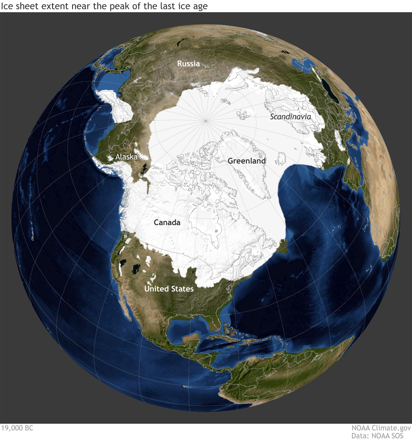
In those 800K years, the Earth has experience cycles of glaciation/deglaciation with recurring ice ages. Figure (\PageIndex{5}\) below shows a depiction of the last ice age which peaked 21,000 years ago (left). At that time, the ice cap over New York City was about 1 mile high (right) as CO2 was at 185 ppm!
 |
 |
By 5000 BCE, the glacier had retreated to more modern levels, leaving ice over the Arctic Ocean, and over Greenland. CO2 levels were then around 260 ppm. A change of just 100 ppm in CO2 was sufficient to lead to the melting of the Northern Hemisphere glaciers. The image above is not "Northern Hemisphere-Centric" since the great glaciers were localized in the Northern Hemisphere in the ice ages. That's because glaciers grow over land and most of the land on the planet is in the Northern Hemisphere. (Our climate studies won't include the time when one continent - Pangea- existed.) The video below shows an animation of the Northern Hemisphere ice shield as it changed with time from 19,000 BCE to now to a projected future that assumes little action to change CO2 emissions. Pay special attention to the graphs which show sea level changes as well.
Best estimates by Tierney et al now show that during the last ice age, the average global temperature was 6 degrees Celsius (11 F) cooler than today, which in the 20th century is 14 C (57 F). The Arctic however was much colder (about 14 C or 25 F). The group also came up with an estimate of climate sensitivity, the increase in temperature with increasing CO2. That value is a rise of 3.4 °C (6.1 °F) for a doubling in CO2. In 1896, Arrhenius, recognizing that CO2 was a greenhouse gas, actually calculated that doubling atmospheric CO2 would cause a rise of 4-5 °C. No one can say we haven't known!
A new value for climate sensitivity giving a rise of 4.8 °C (8.6 °F) for a doubling of CO2 was determined by Hansen et al (2023) using more precise data about temperatures and CO2 concentrations derived from isotopic analyses of ice core samples. If this value holds, the environment needed for human life and our present society is in serious jeopardy unless we take immediate measures to stop emissions and actually cool the planet. In addition, the rate of increase in global and ocean temperatures has accelerated after 2010 and the likely culprit is an actual decrease in toxic SO2 aerosols released by ocean vessels in the North Pacific and Atlantic Oceans and in China from the reduction of dirty coal-burning facilities. Aerosols reflect incident solar light and also increase cloud formation, both of which help cool the planet. Paradoxically, the reduction of anthropogenic aerosols, while great for cardiovascular and pulmonary health, will accelerate global warming. India would be much warmer now if not for the high aerosol concentrations from smog that covers many of its large cities and countryside.
Climate, CO2 and temperature have always changed over geological time, but our present rise in anthropogenic CO2 in such a brief time is unprecedented and has led to CO2 levels that far exceed those during the warmer interglacial periods when Northern Hemisphere glaciers had retreated.
The Ice Ages, CO2 and Temperature
It's not increasing CO2 that is causing any observed increases in temperature. CO2 is going up after temperature increases so we don't have to worry about CO2 levels. It's just a natural process and requires no action to reduce fossil fuel use. Why reduce it if it doesn't cause global warming?
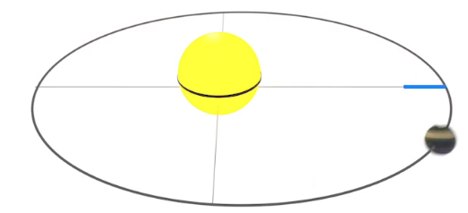
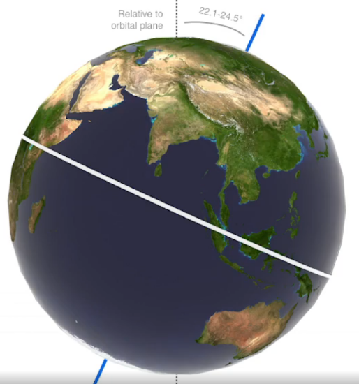
Data and models show that the global increase in temperature is driven mostly by increases in CO2 (and not increasing temperatures driving increasing CO2) as the predominant cause. That begs the question as to what starts the process of deglaciation. It turns out that cyclic increases in solar irradiance that increase temperatures, especially in the Northern Hemisphere, start deglaciation. A prime factor is the changes in the orbital dynamics of the Earth with respect to the sun. As you know, the orientation of the Earth's rotation axis remains generally fixed and pointed in the same orientation as the Earth rotates around the sun. This fixed orientation leads to our annual spring, summer, fall, and winter cycles on Earth. In the winter, the northern hemisphere is pointed away from the sun, leading to decreased solar irradiance per square meter in the Northern Hemisphere, causing winter there. When the Earth is on the opposite side of the sun, the axis points in the same direction but tilts towards the sun, leading to summer in the northern hemisphere. However, the orbital dynamics of the Earth do change in cyclic fashions over long periods of time. These long-term changes in the Earth's orbital shape (eccentricity), tilt (obliquity), and wobble (precession) are called the Milankovitch Cycle, and are illustrated in Figure \(\PageIndex{6}\). These cycles cause small temperature increases that start deglaciation. Click on each image below to download and view very short videos illustrating these orbital changes.
Change in eccentricity (orbital shape) - (100,000 yr cycle)
Change in obliquity (tilt) (41,000 yr cycle)
Axle precession (wobble) (26,000 yr cycle)
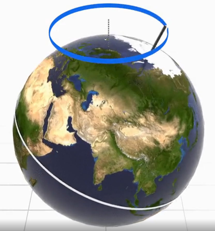
Figure \(\PageIndex{6}\): The Milankovitch cycle showing changes in the Earth's orbital dynamics with respect to the sun. https://climate.nasa.gov/news/2948/m...arths-climate/
Based on these cycles, Milankovitch calculated that recurring ice ages should occur approximately every 41000 years. Ice ages did occur at this interval from about 3 million years ago (MYA) to 1 million years ago (MYA). About 800,000 YA they lengthened to about 100,000 years, which corresponds to the Earth's eccentricity cycle. The increased duration of the cycle led to longer-lasting glaciers which moved further south in the Northern Hemisphere. One likely explanation for the increase in time between ice ages is that repeated glaciation/deglaciation eroded the bedrock in the Northern Hemisphere, converting it to regolith (rocks, soil, and dust). This allowed an increased velocity of movement of the glaciers to the south due to decreased frictional resistance, and thicker ice cap formation (more time to accrue ice), which required a longer time to melt. This also provided a positive feedback loop as the increased northern ice area would reflect more of the sun's energy back into space, cooling the planet. Punctuating these rhythmic orbital and ice age cycles are other events such as large volcanic eruptions, asteroid impacts, etc, that could produce minor to major changes in climate, and resulting mass extinctions.
Figure \(\PageIndex{7}\) shows how a combination of tilt angle, precession axis, and orbital shape at around 200 KYA (narrow rectangle across all the graphs) combined to lead to low glacial ice volume (bottom graph).
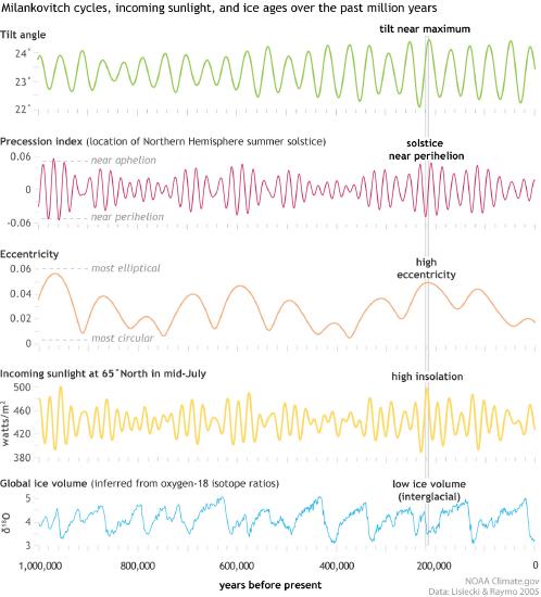
Figure \(\PageIndex{7}\): Milankovitch cycle contribution to ice volume over the past 1M years
If orbital changes (or forcing) trigger deglaciation, what is the role of increasing levels of the greenhouse gas CO2, which clearly covary with temperature (see Fig 3)? Temperature increases derived from orbital and hence solar "forcing" seem to precede CO2 increases for just short periods of time (perhaps 100 - 200 years). After that, CO2 causes almost all of the global increase in temperatures during deglaciation, with CO2 and temperature going up together. A global increase of about 0.3 C due to the Milankovitch cycle leads to greater Northern Hemisphere irradiance. This causes localized and limited melting of the Northern ice shield, leading to increases in ocean temperatures in the northern oceans. These increases slow a major ocean current (the Atlantic Meridional Overturning Circulation - AMOC) which inhibited the burial and return of cold water in tropical and southern oceans. This in turn led to a warming in the south accompanied by the release of large amounts of CO2 stored in the oceans (see Carbon Cycle in 31.3). The release of this greenhouse gas was then responsible for most of the warming that lead to massive deglaciation. This "interhemispheric see-saw" transfer of heat from the north waters to the southern waters is key. For the far majority of the warming during glacial melting, CO2 and temperature change synchronously.
Interpreting climate data is difficult. For example, it was found through measuring 15N/14N ratios that gases like N2 and by extension CO2 could rapidly diffuse through the compacting snow (firn, comprising the top 50-100 meters of the ice cap) until it became trapped in the solid ice beneath it. This would lead to the presence of "newer" CO2 in older ice samples, and the conclusion the temperature changes preceded changes in CO2. Corrections are made to the data to address the "apparent" time shift.
The CO2 trapped in bubbles in the ice core samples from Antarctica reflects global CO2 levels given atmospheric circulation but the temperatures measured from the same core samples (see Chapter 31.2) represent local (Antarctic) temperatures. Ice core samples from Greenland and ocean sediment samples from around the world are used to measure temperature at different locations over time. All of these data are required to model climate. Combined they lead us to our present interpretation of the linkage of CO2 and temperature rise over time.
Increased solar irradiance on Earth arising from cyclic changes in the Earth's orbit leads to short, small temperature increases in the North Hemisphere. These lead to the release of the greenhouse gas CO2 from the oceans, which causes synchronous warming of the planet and subsequent deglaciation.
So when skeptics say that temperature increases preceded CO2 increases, you can acknowledge they did but that the bulk of the warming is attributed to increasing CO2 released from ocean stores which leads to synchronous temperature increases and deglaciation. Using the words of chemistry, small temperature increases from orbital forcing catalyzed the release of huge amounts of CO2 dissolved in the ocean. In Chapter 31.3 we will explore the carbon cycle in more detail and look at how it affects CO2 levels.
Termination of the Ice Ages
How did the ice ages terminate? Contributions from the orbital forcing derived from the Milankovitch cycle play a part. Another factor seems to be dust derived from regolith, itself made by glacier movement as we mentioned above. How can that hypothesis be tested? By using proxies for dust, namely iron and long-chain n-alkanes (derived from plant waxes) that have been deposited in sediments. First, let's look at a graph of CO2 and temperature changes and superimpose those on iron and long-chain fatty acid levels, as shown in Figure \(\PageIndex{8}\).
 |
 |
A close examination of the two vertically aligned graphs from around 120 K to 130 KYA shows that the iron and n-alkane depositions are at a minimum at the same that CO2 and temperature are peaking! What explains this negative correlation? It depends on the intimate connection of the biosphere with the nonbiological world (an arbitrary distinction).
Iron and n-alkanes are circulated and delivered in dust. The long-chain alkanes, highly abundant in waxes and enriched in odd carbon number chains, were presumably derived from leaf waxes which prevent water loss from plants, especially during higher temperatures. Dust deposits were first observed in geological time in the switch from the warmer Pliocene (5.3 to 2.6 MYA) to the Pleistocene (2.6 MYA to 11.7KYA, see Fig 8 below). During the warmer Pliocene, the difference in global and atmospheric temperatures was lower, and with this smaller temperature gradient, winds that could globally transfer dust would be diminished. Also, the warmer Pliocene (5.3 to 2.6 MYA) would have more rain, which would have removed dust from the global circulation.
As temperatures cooled in the Pleistocene (2.6 MYA to 11.7KYA), cycles of glaciation would produce more dust-containing regolith (rocks, soil, and dust), which would be dispersed through stronger global winds from higher temperature gradients and less rain. Dust contains carbon (for example long chain fatty acids) and perhaps more importantly iron, which is needed for oceanic phytoplankton growth. Without Fe, the uptake of CO2 by phytoplankton (primary production) would not occur, leading to increased CO2 in the atmosphere. Stronger regional atmospheric winds would lead to increased upwelling of nutrients as well as deep ocean CO2. The CO2 would enter the atmosphere more readily in the absence of dust deposition of iron.
In summary:
- High CO2 and high temperature (lower global temperature gradients, more rain) are associated with low dust, as measured with the proxies Fe and n-alkanes). Low dust leads to low deposition of Fe and n-alkanes in the ocean, which decreases phytoplankton primary production, the fixing of CO2 into biomass), leading to increased CO2 movement from the ocean to the atmosphere, increasing temperature. This is an example of a positive feedback loop (higher temperatures leading to higher temperatures.
- Low CO2 and low temperature (higher global temperature gradients, stronger winds, less rain) are associated with high dust with Fe and n-alkanes deposition. This increases phytoplankton primary production and decreases CO2 movement from the ocean to the atmosphere, in a negative feedback loop.
By the end of a glacial deposition cycle, dust, blown by stronger winds from higher temperature gradients, was increasingly deposited on the ice sheets. Along with leading to more heat absorption by the sheets, it would also decrease their reflectivity (albedo). Both effects would promote ice sheet melting. Also, a cooler planet during glacial maximum had less precipitation, which along with lower CO2, would lead to more plant and tree death, increasing soil erosion and desertification, both effects which would have increased dust production and its deposition on ice sheets. Then when CO2 rose to 280 ppm, plant life renewed itself, and dust levels dropped.
Climate change from 66 million years ago to now
Antarctic ice core data are now available for the past 2 M years. Ocean sediment data can be used to go back even further in time to 66 million years ago (MYA) just before the dinosaurs died after the massive asteroid impact forming the Chicxulub crater buried underneath the Yucatán Peninsula in Mexico. A brief review of geological eras, periods and epochs is shown below in Figure \(\PageIndex{9}\)
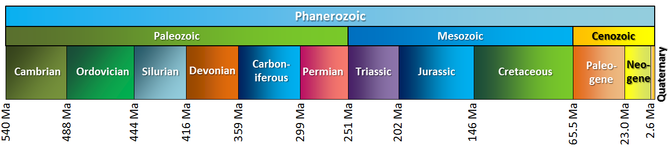
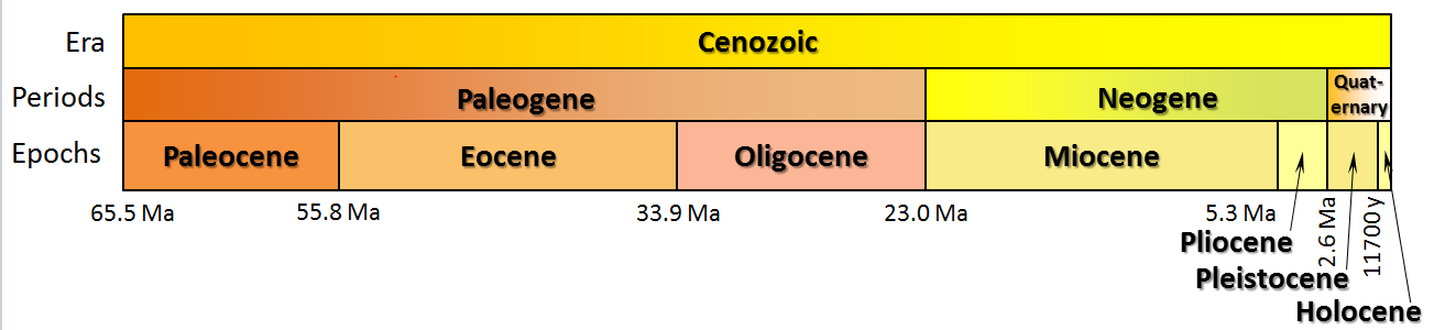
Figure \(\PageIndex{9}\): Geological Era, Periods and Epochs
CO2 levels and associated temperatures derived from ocean sediment cores going back to 66 MYA are shown in Figure \(\PageIndex{10}\).
V3GraphCO2_T.svg?revision=1&size=bestfit&width=957&height=574)
Figure \(\PageIndex{10}\) CO2 levels (red) and temperatures (blue) derived from ocean sediment cores going back to 66 MYA = 66,000 KYA . Data from Rae et al. Annual review of Earth and planetary sciences, 49, 2021
Note again the parallel rise and fall of CO2 and temperature. Eventually, they fall further in the Pliocene (5.3 to 2.6 MYA) and Pleistocene (2.6 MYA to 11.7KYA) epochs with cyclic glacier/interglacial periods we've discussed above. It wasn't until the late Miocene (10 to 6 MYA) that Northern hemisphere glaciation started and both poles of the planet had glacial sheets.
The time frame shown in Figure 9 encompasses the Cenozoic era (65 MYA when the dinosaurs died to about now). CO2 levels were much higher than today in the greenhouse Paleocene and Eocene eras but decreased to about 500 ppm in the Oligocene (34 MYA). An almost stepwise drop in CO2 and temperature occurred in the Eocene to Oligocene transition (EOT), about 33 MYA. Data shows the development of large ice sheets appearing on Antarctica at this time. Before the EOT (33 MYA), Antarctica was ice-free, as shown in the recreation in Figure \(\PageIndex{11}\).
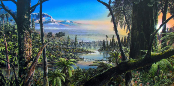
Figure \(\PageIndex{11}\): Reconstruction of the West Antarctic mid-Cretaceous temperate rainforest. Image credit: J. McKay / Alfred-Wegener-Institut / CC-BY 4.0. https://www.sci.news/othersciences/p...ing-09921.html
Proxy data for temperatures show that the transition was most likely caused by a decrease in CO2 and some orbital forcing was probably involved. Present models still struggle to explain the EOT (33 MYA) transition, but it is clear that both CO2 and temperature decreased. Where did the CO2 go? Most assuredly into the oceans.
To understand that, we have to understand a bit about the carbon cycle, which we will discuss more fully in the next chapter section. Let's briefly discuss the role of atmospheric CO2 and its interaction with the ocean. The main gases in the atmosphere, N2 and O2, are found in very low concentrations in the ocean since they are nonpolar and generally unreactive. CO2 is also a nonpolar trace gas, but in contrast, it can readily react with water to form HCO3- and CO3-2, which are found in great abundance in ocean reserves. Hence the ocean chemistry of CO2 determines in large part the levels of atmospheric CO2. The coupled reactions of CO2 are shown below.
\begin{equation}
\mathrm{CO}_2(\mathrm{~g}, \mathrm{~atm}) \leftrightarrow \mathrm{CO}_2(\mathrm{aq}, \text { ocean) }
\end{equation}
\begin{equation}
\mathrm{CO}_2(\mathrm{aq} \text {, ocean })+\mathrm{H}_2 \mathrm{O}(\mathrm{I} \text {, ocean }) \leftrightarrow \mathrm{H}_3 \mathrm{O}^{+}(\mathrm{aq})+\mathrm{HCO}_3^{-}(\mathrm{aq})
\end{equation}
\begin{equation}
\mathrm{H}_2 \mathrm{O}(\mathrm{I})+\mathrm{HCO}_3^{-}(\mathrm{aq}) \leftrightarrow \mathrm{H}_3 \mathrm{O}^{+}(\mathrm{aq})+\mathrm{CO}_3{ }^{2-}(\mathrm{aq} \text {, sparingly soluble })
\end{equation}
This chemistry helps determine the pH of the ocean. Figure \(\PageIndex{12}\) shows atmospheric levels of CO2 and ocean pH over the last 66 million years.
V3GraphCO2_pH.png?revision=1&size=bestfit&width=963&height=577)
Figure \(\PageIndex{12}\): Atmospheric levels of CO2 and ocean pH over the last 66 million years
Before the EOT at 34 MYA, atmospheric CO2 levels were higher and ocean pH levels lower (around 7.7). After the EOT (33 MYA), atmospheric CO2 is much lower and ocean pH is higher (more basic, 7.9 rising to 8.1). What happened to the CO2 is a bit unclear. Atmospheric CO2 decreased by moving into the oceans but wouldn't that have lowered the pH based on the chemical equations presented above? It would have but it turns out that the ocean alkalinity is determined not just by H3O+ produced by the equations above, but by the dissolved inorganic carbon ions, HCO3- (aq) and CO32- (aq), which are conjugate bases. Increased HCO3- (aq) and SiO4-2 (aq) from weathering solid carbonates and silicates that entered the oceans would raise the pH of the oceans.
A little review of introductory chemistry helps here.
Let's take bicarbonate, the weak conjugate base of the weak acid carbonic acid. HCO3- can act as both an acid and base.
Rx 1: Acts as an acid: HCO3- (aq) + H2O (l) ↔ H3O+(aq) + CO32- (aq)
\begin{equation}
K_{a 2}=\frac{\left[\mathrm{H}_3 \mathrm{O}^{+}\right]\left[\mathrm{CO}_3^{2-}\right]}{\left[\mathrm{HCO}_3^{-}\right]}=4.7 \times 10^{-11}
\end{equation}
Rx 2: Acts as a base: HCO3- (aq) + H2O (l) ↔ H2CO3 (aq) + OH- (aq)
\begin{equation}
K_{b 2}=\frac{\left[\mathrm{H}_2 \mathrm{CO}_3\right]\left[\mathrm{OH}^{-}\right]}{\left[\mathrm{HCO}_3^{-}\right]}=2.2 \times 10^{-8}
\end{equation}
The equilibrium constant for the reaction of HCO3- as a base is much larger so bicarbonate is a stronger base than acid.
Whatever the mechanism of the CO2 drawdown, it led to decreasing temperatures in the EOT transition. Increased alkalinity of the ocean would also consume H3O+, increasing ocean pH.
A summary of planetary temperatures across geological time is shown in Figure \(\PageIndex{13}\).

Figure \(\PageIndex{13}\): Temperature of Earth over 500 million years. https://commons.wikimedia.org/wiki/F...alaeotemps.png. (Excel available). Creative Commons Attribution-Share Alike 3.0 Unported
There are several key features to note. The last time CO2 was as high as today (415 ppm) was about 3 million years ago. Repetitive cycles of glaciation/deglaciation are obvious in the Pleistocene (2.6 MYA to 11.7KYA).
At around 55 MYA, a spike in temperatures of about 50 - 90F (or even more) on an already warmer planet occurred over about a 100K year timeframe. This is known as the Paleocene/Eocene thermal maximum (PETM). The poles warmed to near 70 0F and alligators and palm trees were found there. The warming also led to the spread of tropic rainforests from the equator, allowing the evolution and proliferation of new plant species including flowering plants and an incredible biodiversity of insects, bird,s and animals that relied on them. Flowering plants produce fruits, which helped drive the evolution of mammals and the first true primates, including the tiny Teilhardina magnoliana. It may have resembled the picture below. (https://en.wikipedia.org/wiki/Teilhardina). Bigs eyes and hands would allow them to find fruit in the tropical forests.

The temperature increase was caused by a dramatic spike in CO2 from deep-sea volcanoes and vents, which also led to a dramatic drop in ocean pH as measured by the loss of deep-sea CaCO3 (chalk). Methane hydrates were also released. These environmental and biosphere changes are visually evident in geological deep-sea sediment records as shown in Figure \(\PageIndex{14}\).

Figure \(\PageIndex{14}\): Overview for the Paleocene–Eocene Thermal Maximum (PETM, 55.5 MYA) data from deep-sea records and the terrestrial Polecat Bench
(PCB) drill core against age. Westerhold et al. Clim. Past, 14, 303–319, 2018. https://doi.org/10.5194/cp-14-303-2018. Creative Commons Attribution 3.0 License
Sediment cores were taken at various sites (1262, 1267, 1266, 1265, 1263, and 690) that are aligned from left to right according to the water depth from deep to shallow. Note at 55.93 million years ago, at the start of the PETM, there was a sharp transition from light brown/gray which is enriched in chalk, to dark brown enriched in clay. Ocean acidification dissolved the chalk. It took over 100,000 years to recover.
This very short time frame is called the Paleocene/Eocene thermal maximum (PETM, 55.5 MYA), which shows very quick spikes (on the geological time scale) can and do occur. Approximately 1.5 petagrams (1015) of CO2 were released annually during the PETM. Now we are releasing about 25 petagram per year. Our present rate of warming is much greater than the rate of warming during the PETM (55.5 MYA). The best candidates for the source of CO2 release that caused the PETM are volcanoes, the oceans, and the permafrost. In addition, methane hydrates (a solid form of methane found in low- temperature high-pressure waters) might also be another factor.
The PETM and time after allowed for optimal evolution of primates. In fact that time might be called the Age of the Primates (analogous to the Age of the Dinosaurs). Figure 13 shows that the arrival of Oligocene was accompanied by much lower temperatures resulting from CO2 drawdown. This decimated the habitat for the primates except for in the tropic rainforests. Primates disappeared completely from North America but thrived in Africa. Tectonic forces caused the generation of the African Rift valley, characterized by diverse geology and a less homogenous and more fractured landscape which again provided new challenges but also new habitats for the evolution of primates and the eventual appearance of Homo Sapiens.
Update from December 3, 2023 Science
In December 2023, a refinement of CO2, temperature, and sea level rise data since the demise of the dinosaurs 65 million years ago was published. (The geological interval from 66 million years ago to now is called the Cenzoic Era, and consists of 3 periods, the Paleogene until 23 MYA, followed by the Neogene until 2.6 MYA, followed by the Quaternary.) A group, the Cenozoic Carbon Dioxide Proxy Integration Project (CenCO2PIP) Consortium, reviewed and reevaluated all "proxy" measurements used to determine past climate conditions (we will discuss proxies using isotope ratios in ice cores and sediments as proxies for actual CO2, temperature, and sea level changes in the next few sections.) The revised data, which represents the best we have, is shown in Figure \(\PageIndex{15}\) below. For this work, pay close attention to graphs A (CO2), B (relative temperature changes) and C (sea level changes). Note that CO2 levels in 2022 were last seen 14 million years ago!
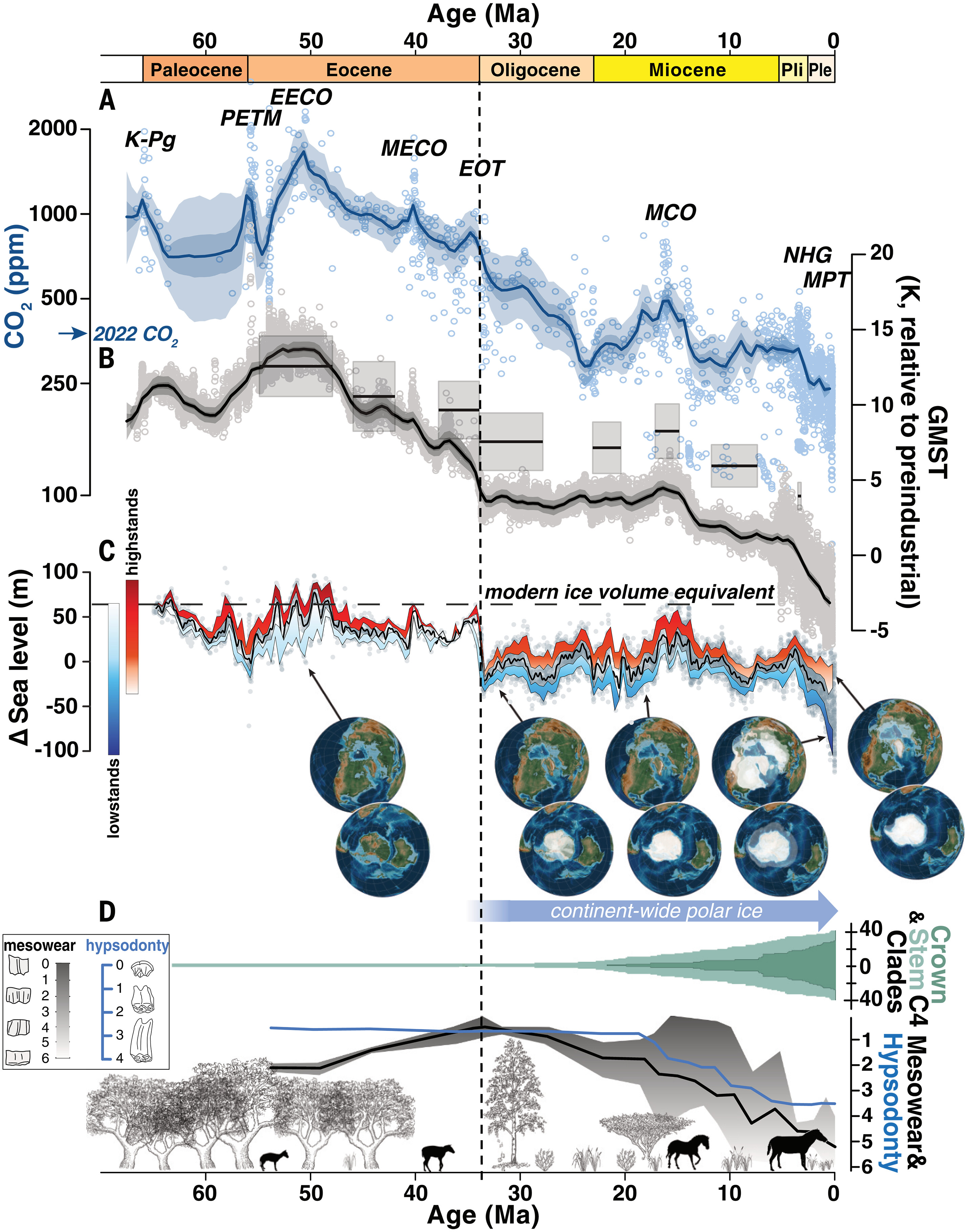
Figure \(\PageIndex{15}\): Category 1 paleo-CO2 record compared to global climate signals. From The Cenozoic CO2 Proxy Integration Project (CenCO2PIP) Consortium, Toward a Cenozoic history of atmospheric CO2.Science382, eadi5177(2023). DOI:10.1126/science.adi5177. Reprinted with permission from AAAS.
The legend below is directly taken from the Science article. The vertical dashed line indicates the onset of continent-wide glaciation in Antarctica.
(A) Atmospheric CO2 estimates (symbols) and 500-kyr mean statistical reconstructions (median and 50 and 95% credible intervals: dark and light-blue shading, respectively). Major climate events are highlighted: K-PG, Cretaceous/Paleogene boundary; PETM, Paleocene Eocene Thermal Maximum; EECO, Early Eocene Climatic Optimum; MECO, Middle Eocene Climatic Optimum; EOT, Eocene/Oligocene Transition; MCO, Miocene Climatic Optimum; NHG, onset of Northern Hemisphere Glaciation; and MPT, Mid-Pleistocene Transition. The 2022 annual average atmospheric CO2 of 419 ppm is indicated for reference.
(B) Global mean surface temperatures estimated from benthic δ18O data following Westerhold et al. (43) (solid line, individual proxy estimates as symbols, and statistically reconstructed 500-kyr mean values shown as the continuous curve, with 50 and 95% credible intervals) and from surface temperature proxies (gray boxes) (45).
(C) Sea level after (66) with gray dots displaying raw data; the solid black line reflects median sea level in a 1-Myr running window. High- and lowstands are defined within a running 400-kyr window, with lower and upper bounds of highstands defined by the 75th and 95th percentiles, and lower and upper bounds of lowstands defined by the 5th and 25th percentiles in each window. Globes depict select paleogeographic reconstructions and the growing presence of ice sheets in polar latitudes from (116).
(D) Crown ages show that C4 clades, with CCMs adapted to low CO2, initially diversified in the early Miocene, and then rapidly radiated in the late Miocene (117). Flora transition from dominantly forested and woodland to open grassland habitats based on fossil phytolith abundance data (96). North American equids typify hoofed animal adaptations to new diet and environment (103), including increasing tooth mesowear (black line; note the inverted scale), hypsodonty (blue line), and body size.
The results reconfirm the strong correlation across geologic time of CO2 and temperature, but there are some time intervals when they were out of synchrony. One example is from 37 to 34 MYA, around the time of the Eocene to Oligocene transition (EOT), described above. In Figure 15, CO2 didn't change much as the earth cooled in the time preceding the EOT. In contrast, there was a big drop in CO2 in the Oligocene as the temperatures remained flat. The start of the Oligocene also showed a big drop (55 m) in sea levels coincident with the EOT, the fall in temperatures, and the rise in glaciation. The authors state that some of the divergences in CO2 and temperatures are likely not related directly to CO2 but other variables such as changes in "paleogeography" arising from continental drift, plate tectonics, etc that might have changed the ocean currents and also changes in reflectivity of sunlight. In addition, the proxies used for those times might have been affected by unaccounted-for changes in seawater composition and pH.
This extensive data presented an opportunity of calculate the climate sensitivity (how much temperature changes with a doubling of CO2) as we discussed above. The value calculated by Tierney was about 3.4 °C (6.1 °F), although Hansen's recent estimate is higher. These values are likely what's called the equilibrium climate sensitivity (ECS) which includes relatively fast feedbacks like cloud cover, sea ice, etc, which act over 100s of years. The value calculated in the new study is not as fine (it courser) with resolutions in 1000s of years, so instead they calculate a much longer-term climate sensitivity called the Earth Systems Sensitivity (ESS) that includes long-term (in geological time) events such as changes in continent-wide ice sheets. The value of ESS of between 5°C (9°F) to 8°C (14.4°F), much higher than the ECS widely accepted for our present time. A doubling of CO2 without some mechanism for drawdown, if sustained over geological time, would transform the world of the distant future. It would be similar to conditions during the Paleocene/Eocene thermal maximum (PETM), when the poles warmed to near 70 0F, conditions that allowed the presence of alligators and palm trees at the poles.
This chapter has been divided into two sections. Got to Chapter 01B: Back to the Present and Future of Climate Change to see where we are and where we are headed!
- Climate change is the long-term change in the average weather patterns on Earth.
- The primary cause of climate change is the burning of fossil fuels, which releases large amounts of greenhouse gases, such as carbon dioxide (CO2), into the atmosphere.
- Greenhouse gases trap heat in the atmosphere, causing the Earth's temperature to rise. This is known as the greenhouse effect.
- The most significant contributor to climate change is CO2, which is released when fossil fuels are burned. Other significant contributors include methane, nitrous oxide, and fluorinated gases.
- Climate change has a wide range of impacts on the Earth's systems, including rising sea levels, changes in precipitation patterns, increased frequency and intensity of extreme weather events, and disruptions to ecosystems.
- The global temperature has already risen by 1 degree Celsius (1.8 degrees Fahrenheit) since the pre-industrial era, with most of the warming occurring in the last few decades.
- The Intergovernmental Panel on Climate Change (IPCC) has stated that limiting global warming to 1.5 degrees Celsius (2.7 degrees Fahrenheit) above pre-industrial levels could significantly reduce the risks and impacts of climate change.
- Reducing greenhouse gas emissions is essential in order to slow or stop climate change. This can be achieved through a combination of actions, such as increasing the use of renewable energy sources, improving energy efficiency, and reducing deforestation.