14.5: Metabolism and Signaling: The Steady State, Adaptation and Homeostasis

Search Fundamentals of Biochemistry

Learning Goals 

(Learning goals written by Claude, Sonnet 4.6, Anthropic)

Response Profiles: Linear, Hyperbolic, and Sigmoidal

• Distinguish among linear, hyperbolic, and sigmoidal steady-state response profiles for a signaling molecule or substrate, derive the steady-state equation for each using mass action or Michaelis-Menten kinetics, and explain the physiological advantages of each profile in terms of sensitivity, dynamic range, and the ability to discriminate signal from noise.
• Explain why embedding a binding interaction or enzyme-catalyzed reaction within a larger pathway can fundamentally alter its apparent response profile, and why maintaining a constant stimulus indefinitely would be biologically harmful in most signaling contexts.

Adaptation and Homeostasis

• Define perfect and near-perfect adaptation operationally — an initial high-magnitude response to a stimulus followed by return to a basal state that is mostly parameter-independent — and explain why the capacity for adaptation is essential for homeostasis at the molecular, cellular, and organismal levels.
• Apply the ASBMB framework for homeostasis to metabolic and signaling pathways, connecting the concepts of steady state, feedback regulation, and energy expenditure to the biological imperative of maintaining narrow concentration ranges for metabolites and signaling molecules.

Molecular Circuits That Generate Adaptation

• Describe the negative feedback loop as a two-node circuit capable of near-perfect adaptation, write the differential equations for the response molecule A and the inhibitor B, and explain how the time-delayed inhibitory feedback dampens the response to repeated or increasing stimuli.
• Describe the incoherent feedforward system as a three-node circuit that achieves near-perfect adaptation by routing the stimulus simultaneously to both the response molecule A and a time-delayed inhibitor B, and explain why the simultaneous activation of both an output and its inhibitor by the same input is described as "incoherent."
• Describe Type A and Type B state-dependent inactivation circuits, explaining how the existence of three conformational states (off, on, and inactivated) in proteins such as voltage-gated Na⁺ channels enables a rapid response followed by a refractory period and eventual return to the activatable resting state.

Recent Updates: 9/13/26

Interactive simulations for the simple motifs for different adaptations are included throughout the chapter.

Introduction

In Chapter 5, we studied binding interactions; in Chapter 6, we studied kinetics; and in this chapter, we studied principles of metabolic control.  We've learned the following:

Binding Reactions

• For simple binding of a ligand to a macromolecule, graphs of fractional saturation of the macromolecule vs. free ligand concentration are hyperbolic and demonstrate saturation binding.  In the initial part of the binding curve, when [L] << K_D, the fractional saturation shows a linear dependence on free ligand concentration.   Figure \(\PageIndex{1}\) shows [ML] vs L, which is the same basic equation as a plot of Y vs L.

Figure \(\PageIndex{1}\)

• For allosteric binding of a ligand to a multimeric protein, graphs of fractional saturation vs free ligand concentration are sigmoidal and also display saturation binding. In the first part of the binding curve, the fractional saturation is much more sensitive to ligand concentration than in simple binding of a ligand to a macromolecule with one binding site.  Figure \(\PageIndex{2}\) below shows graphs for the allosteric binding of a ligand to a macromolecule using the Hill Equation (instead of the MWC equation we used to model O₂ binding to tetrameric hemoglobin).

Figure \(\PageIndex{2}\)

In these two plots, the system (in this case, a single macromolecule) shows different sensitivities to ligand concentration, enabling it to respond differently to changes in physiological conditions.

Binding and Chemical Reactions 

As with binding interactions, we have observed hyperbolic and sigmoidal plots of initial velocity (v₀) vs [substrate] for enzyme-catalyzed reactions. These also allow appropriate responses to a single substrate in a physiological setting.

But what if you put the same macromolecule and ligand into a larger metabolic or signal transduction pathway in vivo? What kinds of responses would they make to a change in input?  As we have just seen in our discussion of the steady state, the ligand or substrate concentration might not change at all as flux continues through the pathway. One could imagine many scenarios with different inputs and optimal outputs.   For example, what if the input (a reactant or small signaling molecule) comes in pulses? Ultimately, a system should return to its basal state since a prolonged response (such as cell proliferation) could harm the organism's health.

Let's examine some simple examples and see how different inputs lead to specific outputs.  We'll construct some very simple reaction diagrams in VCell and see how varying them leads to different outputs.  Here are two simple cases for isolated chemical species and reactions, analogs to the simple binding reactions described above.

Linear Response: A Signal S and a Response R;  S → R

If no enzyme is involved, the rate doubles as the signal (substrate) doubles since dR/dt = k[S] for the first-order reaction.  If S is the stimulus and R is the response,  a plot of R vs S is linear.  Hence, the system responds linearly with increasing S. Here is the simple chemical equation

\begin{equation}
\mathrm{S} \underset{\mathrm{k}_2}{\stackrel{\mathrm{k}_1}{\rightleftarrows}} \mathrm{R}
\end{equation}

As a concrete example, consider the synthesis and degradation of a protein, characterized by the following equation derived from mass action.

\begin{equation}
\frac{d R}{d t}=k_0+k_1 S-k_2 R
\end{equation}

where S is the signal (ex., concentration of mRNA) and R is the response (ex, concentration of the transcribed protein).  A constant k₀ has been added to account for the reaction's basal rate.  (This is a vastly oversimplified way to model a complex process like mRNA translation to a protein, as it omits 100s of steps.)

Here is the simplified derivation under steady-state (SS) conditions, as typically encountered for enzymes embedded in a pathway.

\begin{equation}
\begin{gathered}
\frac{d R_{S S}}{d t}=k_0+k_1 S-k_2 R=0 \\
R_{S S}=\frac{k_0+k_1 S}{k_2}
\end{gathered}
\end{equation}

The equation is a linear function of S.

Hyperbolic Response:  E+S ↔ ES → E + R  

In a simple enzyme-catalyzed reaction with a fixed enzyme concentration, as S increases, the initial velocity saturates.  Hence, there is a limit on the response, so the response R is a hyperbolic function of S.  Increasing S further after saturation won't lead to more R (in a given amount of time).

As a concrete example of this, consider the phosphorylation/dephosphorylation of a protein R.  R_P represents the phosphorylated and active form of the protein R with concentration [R_P].  The reaction is simply written as R ↔ R_P, where R_P is the response.  Mass action shows the total amount of R, R_T = R + R_P.   We can derive a simple mass-action equation.

Here is the chemical equation

\begin{equation}
\mathrm{R}+\mathrm{S} \underset{\mathrm{k}_2}{\stackrel{\mathrm{k}_1}{\rightleftarrows}} \mathrm{R}_{\mathrm{P}}
\end{equation}

Here is the math equation, again for the steady state (SS), when dR_P/dt = 0.  (We derived the same equation for the steady-state version of the Michaelis-Menten equation in Chapter 6.

\begin{equation}
\frac{d R_P}{d t}=k_1 S\left(R_T-R_P\right)-k_2 R_P
\end{equation}

Derivation: Steady-State Hyperbolic Response to a Stimulus S 

Click below to see the derivation

Derivation

\begin{equation}
\frac{d R_P}{d t}=k_1 R[S]-k_2 R_P
\end{equation}

Then, in the steady state:

\begin{equation}
\begin{gathered}
\frac{d R_P}{d t}=k_1 S\left(R_T-R_P\right)-k_2 R_P=0 \\
k_2 R_{P, S S}=k_1 S\left(R_T\right)-k_1 S\left(R_{P, S S}\right) \\
k_2 R_{P, S S}+k_1 S\left(R_{P, S S}\right)=k_1 S\left(R_T\right) \\
R_{P, S S}\left(k_2+k_1 S\right)=k_1 S\left(R_T\right)
\end{gathered}
\end{equation}

Finally, we get

\begin{equation}
R_{P, S s}=\frac{k_1 S\left(R_T\right)}{\left(k_2+k_1 S\right)}=\frac{\left(R_T\right) S}{\left(\frac{k_2}{k_1}+S\right)}
\end{equation}

In the steady state, dR_P/dt = 0, and the steady-state equation can be written as:

\begin{equation}
R_{P, s s}=\frac{k_1 S\left(R_T\right)}{\left(k_2+k_1 S\right)}=\frac{\left(R_T\right) S}{\left(\frac{k_2}{k_1}+S\right)}
\end{equation}

Sigmoidal Response

Consider this simple reaction for a homotetramer in which each monomer can bind a substrate S:  nS + E_n  ↔ E_nS_n → E_n + nR:  If E_n is a multimeric allosteric enzyme, as S increases, the initial velocity also saturates, but the response R is a sigmoidal function of S (in analogy to the above example).  The equation is too complicated to derive here, but the result reproduces a sigmoidal curve for the steady state, much as the Hill equation does for cooperative binding.

Adaptation and Homeostasis

The above examples show that the response of proteins or enzymes to increasing levels of a stimulus, such as a ligand or substrate, can be linear, hyperbolic, or sigmoidal, with varied outcomes.  However, an ever-increasing or increasing-and-plateauing response might be too much in many biological conditions.  The cell needs a way to turn off the response and return to a basal state, even when stimuli are constant or changing.  This allows a system to adapt to a stimulus and maintain homeostasis. Every system needs to be able to respond and return to a homeostatic basal level.  Maintaining homeostasis is critical to life. 

Homeostasis - ASBMB

The American Association for Biochemistry and Molecular Biology (ASBMB) describes homeostasis and evolution as key underlying concepts in all of biology.  Homeostasis shapes both form and function at the molecular and organismal levels. Homeostasis is needed to maintain biological balance.  Steady states at the molecular and organismal levels in metabolic and signaling pathways are a hallmark of homeostasis. Here are the learning goals for homeostasis designated by the ASBMB 

1.  Biological need for homeostasis

Biological homeostasis is the ability to maintain relative stability and function as the internal or external environment changes. Organisms are viable under a relatively narrow set of conditions. As such, organisms must tightly regulate metabolite and small-molecule concentrations at the cellular level to survive. To optimize resource use and maintain conditions, the organism may sacrifice efficiency for robustness. The breakdown of homeostatic regulation can contribute to the cause or progression of disease or lead to cell death.

2. Link steady-state processes and homeostasis

A system that is in a steady state remains constant over time, but that constant state requires continual work. A system in a steady state has a higher level of energy than its surroundings. Biochemical systems maintain homeostasis via the regulation of gene expression, metabolic flux, and energy transformation but are never at equilibrium.

3. Quantifying homeostasis

Multiple reactions with intricate networks of activators and inhibitors are involved in biological homeostasis. Modifications of such networks can lead to the activation of previously latent metabolic pathways or even to unexpected interactions between components of these networks. These pathways and networks can be mathematically modeled and correlated with metabolomics data and kinetic and thermodynamic parameters of individual components to quantify the effects of changing conditions related to either normal or disease states.

4. Control mechanisms

Homeostasis is maintained by a series of control mechanisms functioning at the organ, tissue, or cellular level. These control mechanisms include substrate supply, activation or inhibition of individual enzymes and receptors, synthesis and degradation of enzymes, and compartmentalization. The primary components responsible for the maintenance of homeostasis can be categorized as stimulus, receptor, control center, effector, and feedback mechanism.

5. Cellular and organismal homeostasis

Homeostasis in an organism or colony of single-celled organisms is regulated by secreted proteins and small molecules, often functioning as signals. Homeostasis in the cell is maintained by regulation and by the exchange of materials and energy with its surroundings.

In the rest of the chapter, we will describe chemically and mathematically simple biological circuits/motifs that allow perfect or near-perfect adaptation to a stimulus, a hallmark of homeostasis.  We define adaptation as a complete or almost complete return to a basal state after introducing a stimulus.  In all the cases below, we will consider not a single application of a stimulus but a pulse application (a repetitive step-function).  The pulsed stimuli could be of constant magnitude or of an increasing or decreasing signal, such as a substrate.  All responses must be transient to avoid uncontrolled responses such as proliferation (a hallmark of tumor cells) or cell death.

Adaptation is commonly found in sensory systems such as vision, hearing, pressure, and taste.  Think of eating your favorite cookie. The first bite is delicious, but by the tenth bite, the positive sensory response is significantly attenuated, which helps keep most people from eating a whole box of cookies in one sitting.

Ma et al. simulated three-component/node (protein, enzyme) systems to identify which might exhibit the potential for perfect or near-perfect adaptation.  The simple 3-component motifs or circuits were modeled using mass-action kinetic equations, ordinary differential equations (which we learned to write in Chapter 6.2), or a combination of both.  The systems that displayed adaptation had to conform to three criteria:

1. The stimulus had to induce a response of high magnitude initially
2. The system had to return to a basal or near-basal state.
3. The return to a basal state had to be mostly parameter-independent.  That is, the return to the basal state must occur across many different parameter combinations.

The possible 3-component components (nodes) and the links among the nodes are shown in Figure \(\PageIndex{3}\) below.

Figure \(\PageIndex{3}\):  Possible 3-component components (nodes) and the links among the nodes.  After Ma et al. Cell Theory,138, 760-773 (2009) https://www.cell.com/fulltext/S0092-8674(09)00712-0.  DOI:https://doi.org/10.1016/j.cell.2009.06.013.

Of over 16,000 models, several hundred met the criteria. Most were variations of simple motifs shown below. The most common motifs were the negative feedback loop and the incoherent feedforward system. 

Much of the discussion, models, and equations used below are from two articles:

• John J Tyson, Katherine C Chen, Bela Novak, Sniffers, buzzers, toggles and blinkers: dynamics of regulatory and signaling pathways in the cell, Current Opinion in Cell Biology, Volume 15, Issue 2, 2003, Pages 221-231, https://doi.org/10.1016/S0955-0674(03)00017-6.
• James E. Ferrell, Perfect and Near-Perfect Adaptation in Cell Signaling, Cell Systems, Volume 2, Issue 2, 2016, Pages 62-67, https://doi.org/10.1016/j.cels.2016.02.006.

Adding a third component to form a mini pathway can change the response R to a stimulus S from linear or hyperbolic/sigmoidal in the steady state to one that exhibits perfect or near-perfect adaptation. We also see this kind of response in signaling pathways in sensation and in chemotaxis, where a cell moves toward a stimulus (a chemoattractant molecule).

Simple 3-node motif/circuit for perfect adaptation

Figure \(\PageIndex{4}\) below shows our first example of a 3-component system that displays perfect or near-perfect adaptation.  The right-hand side shows a VCell reaction diagram. In this example, a stimulus S (a reactant, neurotransmitter, mRNA, etc.) leads to the synthesis of X and R, a response molecule.  Both X and R get degraded.  The yellow squares represent the nodes through which the flux of S to X and R proceeds.  Each node has an equation for the flux, J, through the node.  The left part of Figure 4 shows the periodic pulse of stimulus S, which increases the concentration of S from an initial value of S₀ = 1 μM to S + 0.2 μM at each step. Note that the flux equations for J are very simple and are based on mass action and are not derived through Michaelis-Menten kinetic equations.

Figure \(\PageIndex{4}\):  Simple 3-component system that displays perfect or near-perfect adaptation.

Note that S, the stimulus (or substrate, for example), is a square-wave step function varying from 0 to 1 over the time interval shown in the graph.  The dotted blue line simply shows when the pulse is delivered.  The initial S concentration is 1 μM and increases by 0.2 μM for each step (as shown in the gray line).  Thus, S increases stepwise.

Figure \(\PageIndex{5}\) below is a time-course graph that shows the stepwise (=0.2 uM) increase in S from 1 μM and the concentration of R (the response) over 20 seconds.  Even though S continues to increase in a stepwise fashion, R rises substantially only from the initial input of S (1 μM), and subsequent increases in S with each increment of S are damped out!

Figure \(\PageIndex{5}\): Time course for a 3-component Perfect Response system.  Model by ModeBrick from VCell: CM-PM12648679_MB4:Perfect_Adaptation; Biomodel 188456707

Figure \(\PageIndex{6}\) below is an interactive simulator for this perfect-adaptation model.

Figure \(\PageIndex{6}\): Time course for a 3-component Perfect Response system.  Graph produced using Claude (Anthropic) from a model by ModeBrick using VCell: CM-PM12648679_MB4:Perfect_Adaptation; Biomodel 188456707.  Click Reset to Model Defaults if graphs disappear between runs.

Negative Feedback Loop

The negative feedback loop is one of the simplest circuits/motifs for generating perfect or near-perfect adaptation.  It has only two nodes (yellow dots) and two proteins. An example is bacterial chemotaxis. Figure \(\PageIndex{6}\) below shows a VCell reaction diagram (left), another representation (middle), and the time course graphs for all species. This model works especially well with specific parameter values.

Figure \(\PageIndex{7}\)

Figure \(\PageIndex{7}\):  Near-Perfect Adaptation from Negative Feedback. Adapted from Ferrell (ibid)

The gray line in the graph is the stimulus S (substrate).  The blue line is the response, designated in this model as A.  B acts as an inhibitor (note the dotted line to the input node in the left diagram and the blunt-ended red bar in the middle diagram.  Note that the stimulus goes from 0.2 μM (initial concentration) at t=0 to 1 μM (a 5-fold increase) at 40 seconds, but the response A increases at most from 0.4 (initial condition) to 0.5 (a 1.25-fold increase).

If we say [A] is the output, then the differential equation for dA/dt is given by

\begin{equation}
\frac{d A}{d t}=k_1 \operatorname{S} \cdot(1-A)-k_2 A \cdot B
\end{equation}

dB/dt is given by

\begin{equation}
\frac{d B}{d t}=k_3 A \frac{1-B}{K_3+1-B}-k_4 \frac{B}{K_4+B}
\end{equation}

The constants for the graph (right) produced by the VCell model are:

• k₁ = k₂ = 200
• k₃ = 10; k₄ = 4
• K₃ = K₄ = 0.01

Figure \(\PageIndex{8}\) below is an interactive simulator for Near-Perfect Adaptation from Negative Feedback.

Figure \(\PageIndex{8}\): interactive simulator time course for Near-Perfect Adaptation from Negative Feedback.  Graph produced using Claude (Anthropic) from a model by ModeBrick using VCell.  Adapted from Ferrell (ibid.).  Click Reset to Model Defaults if graphs disappear between runs.

Incoherent Feedforward Systems

In this circuit/motif, the stimulus S increases the concentration of A (the output) but also forms a negative modulator, B, which, with a bit of a time lag, decreases A through inhibition.  This simple system has no feedback inhibition from A. If you're reading carefully, you'll see that the reaction scheme and inhibition are identical to the first circuit/motif we introduced.  Here, we simplify the diagram and give it an official name.  The word incoherent in the name makes sense since the stimulus S is converted both to the output A and to the inhibitor B, which on the surface seems like a crazy (incoherent) thing to do.

Figure \(\PageIndex{9}\) below shows the VCell reaction diagram (left) and a more classical reaction diagram (middle), and progress curves showing S, the stimulus, A, the output or response, and B, the inhibitor.  The dashed line in the left diagram from B to the reaction node for the S → A reaction shows that B affects the rate of that reaction. The equations account for B's inhibitory effects.

 

Figure \(\PageIndex{9}\):  Near-Perfect Adaptation from an Incoherent Feedforward System. Adapted from Ferrell (ibid)

Note that the response A goes up or down a bit with each new step in the concentration of S, but to a very minimal degree. The system is certainly almost perfectly adapted.

The differential equation for dA/dt (where A is the response) is

\begin{equation}
\frac{d A}{d t}=k_1 \operatorname{S} \cdot(1-A)-k_2 A \cdot B
\end{equation}

The equation for dB/dt (the inhibitor generated from A) is

\begin{equation}
\frac{d B}{d t}=k_3 \text { S } \frac{1-B}{K_3+1-B}-k_4 B
\end{equation}

The constants for the graph (right) produced by the VCell model are:

• k₁ = 10; k₂ = 100
• k₃ = 0.1; k₄ = 1
• K₃ = 0.001

Figure \(\PageIndex{10}\) below is an interactive simulator for Near-Perfect Adaptation from an Incoherent Feedforward System.

Figure \(\PageIndex{10}\):  interactive simulator time course for Near-Perfect Adaptation from an Incoherent Feedforward System.  Graph made by Claude (Anthropic).  Click Reset to Model Defaults if graphs disappear between runs.

Notes:  The incoherent feedforward signature is evident.  A (blue) shows a sharp transient spike at each step in S, then relaxes almost all the way back down each time (near-perfect adaptation), while B (orange) tracks S proportionally without any spike, since it's driven directly by S rather than through A.  S drives A directly, and separately drives B (through its own saturable branch that depends only on S and B — B never senses A at all), and B inhibits A's production. That's the key structural difference from the negative-feedback model: there, B was downstream of A and looped back; here, B is a parallel branch off S, not a loop

State-dependent Inactivation Systems.

After initial analyses showed all possible interactions in a 3-component system (see Figure 3), two simple circuits/motifs in this system were identified.  The motif was patterned after protein inhibition in neuronal stimulation, specifically ion channels in neural cell membranes that open in response to changes in transmembrane potential but then close quickly to avoid constant neuronal stimulation (or inhibition).  The Na⁺ ion channel has both fast (1-2 ms) and slow (100 ms) inactivation mechanisms.  The fast one allows repetitive firing, action-potential development, and control of neuronal excitation and neuromuscular junction transmission.  Chapter 28.9 discusses neuronal signaling.  Figure \(\PageIndex{11}\) below shows a simplified model for one type of inactivation of the Na⁺ ion channel

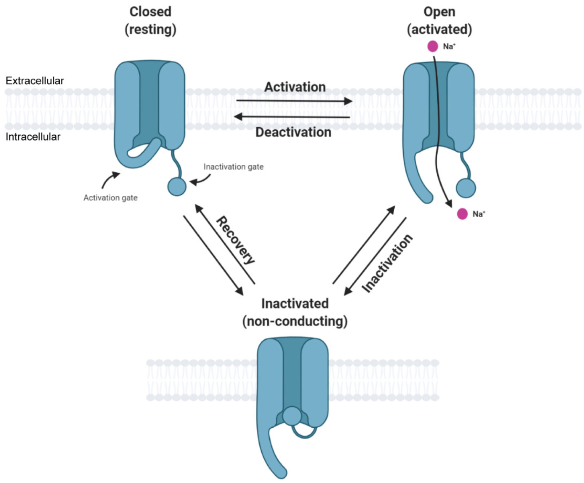
Figure \(\PageIndex{11}\): Simplified state transition model of voltage-gated sodium channels featuring closed, open, and inactivated states.  Zybura, A. et al. Cells 2021, 10, 1595. https://doi.org/10.3390/cells10071595.   Creative Commons Attribution (CC BY) license (https://creativecommons.org/licenses/by/4.0/).

The figure implies at least three conformational states of the channel, so the inactivation of the channel and the circuit/motif for adaptation that we will discuss are called state-dependent inactivations.  The slow return to the original state is observed in many ion channels and in the return of G protein-coupled receptors to the normal state after desensitization.  Some protein kinases (which use ATP to phosphorylate protein substrates) can also be inactivated by internalizing the membrane kinase into vesicles, which can be reactivated and slowly returned to the plasma membrane.

For the construction of a perfect or near-perfect adaptation state, we will assume the protein A exists in an off state (A_off) which binds the stimulus (B or S), an on state (A_on) which is viewed as the response (or A produces the response), and an inactivated state (A_in) which slowly reverts to the A_off state, which can be activated again.  The inactive state can arise from conformational transitions within the protein itself or from another molecule produced downstream in a metabolic or signaling pathway. For example, a GPRC could be phosphorylated or bind another species to become inactive.

Two different circuits/motifs can produce state-dependent inactivation. We'll refer to these as Type A and Type B.

Type A

Figure \(\PageIndex{12}\) shows the VCell reaction diagram (top left), a classical reaction diagram (bottom left), and time course graphs for Type A state-dependent inactivation.

Figure \(\PageIndex{12}\):  Perfect Adaptation for Type A State-Dependent Inactivation. Adapted from Ferrell (ibid).

A_on represents the protein's active state.  This mechanism applies well to the Na⁺ channel. The differential equations for dA_on/dt and dA_off/dt are shown below.

For dA_on/dt

\begin{equation}
\frac{d A_{o n}}{d t}=k_1 \operatorname{Input} \cdot\left(1-A_{o n}-A_{i n}\right)-k_2 A_{o n}
\end{equation}

dA_in/dt

\begin{equation}
\frac{d A_{i n}}{d t}=k_2 A_{o n}
\end{equation}

with constants k₁ = k₂ = 1.

Again, as with the other cases, the stimulus S is pulsed.  The different colors in the bottom-left reaction diagram imply an inactive, off (red) state and a green, active state, each with different conformations. The graphs were produced using VCell.  A slight anomaly in the Aon graph shows two additional small peaks as the system returns to the basal state.  This contrasts with a single peak that returns to the basal state in a simple exponential fashion, as described in the Ferrell paper.  We are unsure of the source of the discrepancy.

Figure \(\PageIndex{13}\) below is an interactive simulator for Type A state-dependent inactivation.

Figure \(\PageIndex{13}\): interactive simulator time course for Type A state-dependent inactivation. Graph made by Claude (Anthropic).  Click Reset to Model Defaults if graphs disappear between runs.

Notes:  This is built from the exact same reaction network and step function input as before, but the outputs are different.  Instead of a feedback or feedforward loop that returns the system to baseline, it's a three-state receptor pool (Aoff ⇄ Aon → Ain) where the inactivation step has no way back.

Type B

In this case, the periodic stimulus, abbreviated as B, is a binding partner for A_off, which produces an active complex B-A_on.   Figure \(\PageIndex{10}\) below shows the VCell reaction diagram (top left), a classical reaction diagram (bottom left), and time course graphs for Type B state-dependent inactivation.

Figure \(\PageIndex{14}\)

Figure \(\PageIndex{14}\):  Perfect Adaptation for Type B State-Dependent Inactivation. Adapted from Ferrell (ibid)

BA_on represents the active state of the protein bound to B, while BA_in represents the inactive complex.  

The equation of dBA_on/dt for the formation of the active state is  

\begin{equation}
\frac{d B A_{o n}}{d t}=k_1\left(B_{t o t}-B A_{o n}-B A_{i n}\right) *\left(1-B A_{o n}-B A_{i n}\right)-k_2 B A_{o n}
\end{equation}

and the equation for dBA_in/dt for the formation of the inactive state is

\begin{equation}
\frac{d A_{i n}}{d t}=k_2 A B_{o n}
\end{equation}

with constants k₁ = k₂ = 4.

The graphs (note the different time-scale concentrations on the left) show a fairly quick return to the basal state after each stimulus pulse (B).

Figure \(\PageIndex{15}\) below is an interactive simulator for Type B state-dependent inactivation.

Figure \(\PageIndex{15}\): Interactive simulator time course for Type B state-dependent inactivation. Graph made by Claude (Anthropic). Click Reset to Model Defaults if graphs disappear between runs.

Note: This has the same three states (Aoff ⇄ active state → inactivated state), but the binding step has a nonlinear rate law.  Instead of simple mass-action (rate ∝ signal × available), the net flux depends on how far the signal is from the already-occupied fraction (active + inactivated). With this different rate law,  once the occupied fraction exceeds the signal, the flux reverses. So as the signal steps back down, the model actively drains the inactivated pool BAin back out — by the end of the run the responsive pool is essentially fully restored (≈1.0), versus Type A's near-total, permanent collapse (≈0). BAon dips very slightly negative for an instant during recovery, a feature of this rate law that lets the inactivated pool flow back out.

Summary

(Summary written by Claude, Sonnet 4.6, Anthropic)

This chapter integrates quantitative frameworks for binding, enzyme kinetics, and metabolic control analysis into a unified treatment of how biological systems respond to stimuli and return to homeostatic basal states—a capacity fundamental to all living organisms.

The chapter begins by reviewing the three canonical steady-state response profiles that emerge from different molecular architectures. A simple first-order chemical process (S → R, no enzyme) generates a linear response, in which the rate of response production is directly proportional to the stimulus concentration. An enzyme-catalyzed reaction operating under Michaelis-Menten kinetics generates a hyperbolic response, with saturation placing an upper limit on the output regardless of the amount of stimulus applied — as illustrated by the phosphorylation/dephosphorylation of a protein substrate. An allosteric, multimeric enzyme generates a sigmoidal response, which is more sensitive to stimulus concentration in a narrow range and allows sharper switching behavior. These three profiles parallel the binding curves discussed in Chapter 5 and the velocity-substrate curves of Chapter 6, and they reflect how the same molecular components can produce fundamentally different physiological behaviors depending on their kinetic architecture.

However, an ever-increasing or plateauing response is biologically untenable in most signaling contexts: prolonged activation drives pathological outcomes ranging from sensory overload to uncontrolled cell proliferation. The cell, therefore, requires circuits that return to a basal state after a stimulus — a property called adaptation — and the maintenance of this basal state across varying conditions is the molecular basis of homeostasis. The ASBMB framework frames homeostasis as a property operating from the molecular to the organismal level, requiring continual energy expenditure to maintain a steady state above thermodynamic equilibrium, and its breakdown is associated with disease progression and cell death.

The chapter then analyzes the minimal molecular circuits capable of generating adaptation. Drawing on computational simulations by Ma et al. of over 16,000 three-node systems, two principal motif families emerge as sufficient for perfect or near-perfect adaptation: negative feedback loops and incoherent feedforward systems.

In the negative feedback loop, the stimulus S activates a response molecule A, which in turn produces an inhibitor B that feeds back to suppress further activation. The two coupled differential equations (dA/dt driven by S and inhibited by B; dB/dt driven by A) produce dynamics in which an initial stimulus triggers a transient spike in A, which is then damped by accumulating B, returning A to near its basal level even as S remains elevated. This motif underlies bacterial chemotaxis and many receptor desensitization phenomena.

In the incoherent feedforward system, S simultaneously drives the synthesis of both A (the response) and B (an inhibitor of A's production). The word "incoherent" reflects the seemingly contradictory logic of a stimulus activating both a response and its own inhibitor — yet this architecture generates robust adaptation because the time lag between A's activation and B's accumulation allows the transient response, while B's eventual inhibitory effect returns A to baseline. The result is a sharp, transient output that scales only weakly with repeated or increasing stimuli.

State-dependent inactivation circuits extend this logic to proteins that can occupy three distinct conformational states — off (resting, activatable), on (active, generating the response), and inactivated (refractory, unable to be reactivated until converted back to the off state). This motif is exemplified by voltage-gated Na⁺ channels, which open rapidly upon membrane depolarization (off → on) but then inactivate within milliseconds (on → inactivated) and recover slowly (inactivated → off), enabling repetitive action potential firing without sustained depolarization. Two variants are presented: Type A, in which the stimulus directly drives the off → on → inactivated transitions within a single protein; and Type B, in which the stimulus (B) forms an active complex B-A_on that transitions to an inactive complex B-A_in. Both produce time-course graphs consistent with rapid response and clean return to the basal state following each stimulus pulse. VCell computational models with mass-action and Michaelis-Menten kinetic equations reproduce these behaviors, reinforcing the conclusion that these simple circuit architectures are sufficient — and necessary — for the adaptive responses that underlie sensory perception, signal transduction, and cellular homeostasis.