9.4: DNA Microarrays

Search Fundamentals of Biochemistry

Learning Goals

(Learning goals written by Claude, Sonnet 4.6, Anthropic)

Microarray Principles and Design

• Explain the molecular basis of DNA microarray technology — describing how each feature (spot) on a microarray contains thousands of identical single-stranded probe oligonucleotides (20–60 nt) complementary to a target gene sequence, how mRNA extracted from cells is reverse-transcribed to cDNA and fluorescently labeled, how labeled target sequences hybridize to complementary probes under high-stringency conditions through Watson-Crick base pairing, how non-specifically bound sequences are washed away, and how the fluorescence intensity at each spot quantifies the relative abundance of the corresponding transcript — connecting stringency (temperature, salt concentration) to the specificity of probe-target base pairing.
• Compare spotted and in situ synthesized oligonucleotide microarray fabrication methods — distinguishing spotted arrays (pre-synthesized oligonucleotide, cDNA, or PCR product probes deposited by robotic pins onto glass slides, low cost, highly customizable but potentially lower sensitivity and reproducibility) from photolithographic oligonucleotide synthesis arrays (Affymetrix 25-mers built directly on silica wafers one nucleotide at a time using light-activated chemistry and masks or digital micromirrors; Agilent 60-mers for higher specificity) — and explain why longer probes provide greater target specificity while shorter probes allow higher feature density and lower manufacturing cost.

Experimental Design and Data Analysis

• Distinguish two-color (dual-channel) from single-color (single-channel) microarray experimental designs — explaining that in two-color arrays, cDNA from two conditions (e.g., diseased vs. healthy tissue) is labeled with spectrally distinct fluorophores (Cy3, λem ≈ 570 nm/green; Cy5, λem ≈ 670 nm/red) and co-hybridized to the same array, generating ratio-based expression comparisons where green signal indicates higher expression in the Cy3-labeled sample, red in the Cy5-labeled sample, and yellow indicates comparable expression in both — while in single-color arrays each array is exposed to only one labeled sample, providing relative expression data across spots within an experiment but requiring separate hybridizations to compare conditions — and identify the relative advantages of each format (two-color: direct internal comparison, efficient; single-color: no cross-sample contamination within a chip, easier cross-experiment comparisons when batch effects are controlled).
• Describe how microarray data are normalized and interpreted — explaining that fluorescence intensity values at each feature represent relative rather than absolute transcript abundance (due to protocol- and batch-specific biases in amplification, labeling efficiency, and hybridization), that spike-in control RNAs of known sequence and abundance hybridized to control probes on the array provide normalization standards, and that data analysis identifies differentially expressed genes by comparing feature intensities between conditions using ratio analysis or statistical tests — connecting this to applications including identifying genes up- or down-regulated in disease, genotyping by comparative genomic hybridization, and characterizing splice variants through exon-specific probe design.

A DNA microarray (also commonly known as a DNA chip or biochip) is a collection of microscopic DNA spots attached to a solid surface. Scientists use DNA microarrays to simultaneously measure the expression levels of large numbers of genes or to genotype multiple regions of a genome. Each DNA spot contains picomoles (10⁻¹² moles) of a specific DNA sequence, known as a probe (or reporter or oligo). These can be short sections of a gene or other DNA elements used to hybridize a cDNA or cRNA (also called antisense RNA) sample (the target) under high-stringency conditions. Probe-target hybridization is usually detected and quantified by detecting fluorophore-, silver-, or chemiluminescence-labeled targets to determine the relative abundance of nucleic acid sequences in the target. The original nucleic acid arrays were macroarrays approximately 9 cm × 12 cm, and the first computerized image-based analysis was published in 1981. Patrick O. Brown invented it. Figure \(\PageIndex{1}\) shows a schematic of DNA Microarrays.

Figure \(\PageIndex{1}\): Schematic of DNA Microarrays. Image by Thomas Shafee

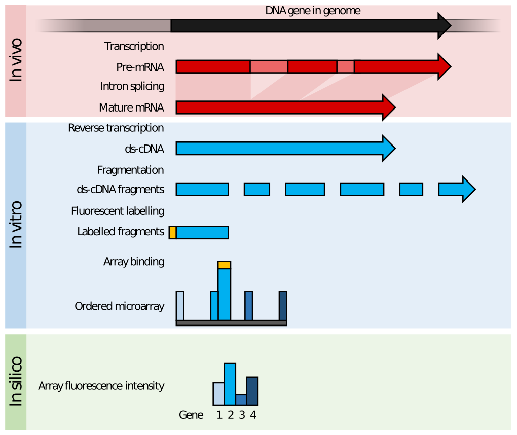
Genes are transcribed and spliced within the organisms to produce mature mRNA transcripts (red). The mRNA is extracted from the organism, and reverse transcriptase copies the mRNA into stable ds-cDNA (blue). In microarrays, the ds-cDNA is fragmented and fluorescently labeled (orange). The labeled fragments bind to an ordered array of complementary oligonucleotides, and measurement of fluorescent intensity across the array indicates the abundance of a predetermined set of sequences. These sequences are typically specifically chosen to report on genes of interest within the organism's genome.

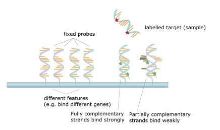
The core principle behind microarrays is hybridization between two DNA strands, a property of complementary nucleic acid sequences that allows them to pair specifically by forming hydrogen bonds between complementary nucleotide base pairs. A high number of complementary base pairs in a nucleotide sequence means tighter non-covalent bonding between the two strands. After washing away non-specifically bound sequences, only strongly paired strands will remain hybridized. Fluorescently labeled target sequences that bind to a probe generate a signal that depends on hybridization conditions (such as temperature) and on washing after hybridization. The total strength of the signal, from a spot (feature), depends upon the amount of target sample binding to the probes present on that spot. Microarrays use relative quantitation, in which the intensity of a feature is compared to that of the same feature under a different condition, and the identity of the feature is determined by its position. Figure \(\PageIndex{2}\) shows the hybridization of target and probe DNA on a microarray.

Figure \(\PageIndex{2}\): Hybridization of Target DNA with the Probe DNA During Microarray Analysis. Image by Squidonius

Many types of arrays exist, and the broadest distinction is whether they are spatially arranged on a surface or coded beads:

• The traditional solid-phase array is a collection of orderly microscopic "spots" called features, each with thousands of identical, specific probes attached to a solid surface, such as glass, plastic, or a silicon biochip (commonly known as a genome chip, DNA chip, or gene array). Thousands of these features can be placed on a single DNA microarray in known locations.
• The alternative bead array is a collection of microscopic polystyrene beads, each with a specific probe and a ratio of two or more dyes. These do not interfere with the fluorescent dyes used on the target sequence.

DNA microarrays can be used to detect DNA (as in comparative genomic hybridization) or RNA (most commonly as cDNA after reverse transcription), which may or may not be translated into proteins. The process of measuring gene expression via cDNA is called expression analysis or expression profiling.

Fabrication

Microarrays can be manufactured differently, depending on the number of probes under examination, costs, customization requirements, and the type of scientific question being asked. Arrays from commercial vendors may have as few as 10 micrometer-scale probes or as many as 5 million or more.

Spotted vs. in situ synthesized arrays

Play media

Microarrays can be fabricated using a variety of technologies, including printing with fine-pointed pins onto glass slides, photolithography using pre-made masks, photolithography using dynamic micromirror devices, ink-jet printing, or electrochemistry on microelectrode arrays.

In spotted microarrays, the probes are oligonucleotides, cDNAs, or small PCR fragments corresponding to mRNAs. The probes are synthesized before deposition on the array surface and are then "spotted" onto glass. A common approach uses an array of fine pins or needles, controlled by a robotic arm, that are dipped into wells containing DNA probes; each probe is then deposited at designated locations on the array surface. The resulting "grid" of probes represents the nucleic acid profiles of the prepared probes and is ready to receive complementary cDNA or cRNA "targets" derived from experimental or clinical samples. This technique is used by research scientists worldwide to produce "in-house" printed microarrays from their labs. These arrays may be easily customized for each experiment because researchers can choose the probes and printing locations on the arrays, synthesize the probes in their labs (or collaborating facility), and spot the arrays. They can then generate labeled samples for hybridization, hybridize them to the array, and scan the arrays with their equipment. This provides a low-cost microarray that can be customized for each study and avoids the cost of purchasing often more expensive commercial arrays that may include vast numbers of genes not of interest to the investigator. Publications indicate that in-house spotted microarrays may not provide the same level of sensitivity as commercial oligonucleotide arrays, possibly owing to small batch sizes and lower printing efficiencies compared to industrial oligo-array manufacturers.

In oligonucleotide microarrays, the probes are short sequences designed to match parts of known or predicted open reading frames. Although oligonucleotide probes are often used in "spotted" microarrays, the term "oligonucleotide array" most often refers to a specific manufacturing technique. Oligonucleotide arrays are produced by printing short oligonucleotide sequences designed to represent a single gene or a family of gene splice variants, by synthesizing these sequences directly onto the array surface rather than depositing intact sequences. Sequences may be longer (60-mer probes such as the Agilent design) or shorter (25-mer probes produced by Affymetrix), depending on the desired purpose; longer probes are more specific to individual target genes, while shorter probes may be spotted at higher density across the array and are cheaper to manufacture. One technique for producing oligonucleotide arrays involves photolithographic synthesis (Affymetrix) on a silica substrate. Light and light-sensitive masking agents are used to "build" a sequence one nucleotide at a time across the entire array. Each applicable probe is selectively "unmasked" before bathing the array in a solution of a single nucleotide. Then a masking reaction occurs, and the next set of probes is unmasked in preparation for exposure to a different nucleotide. After many repetitions, the sequences of every probe become fully constructed. More recently, Maskless Array Synthesis from NimbleGen Systems has combined flexibility with the ability to use many probes. Figure \(\PageIndex{3}\) shows a diagram of a typical dual-color microarray experiment.

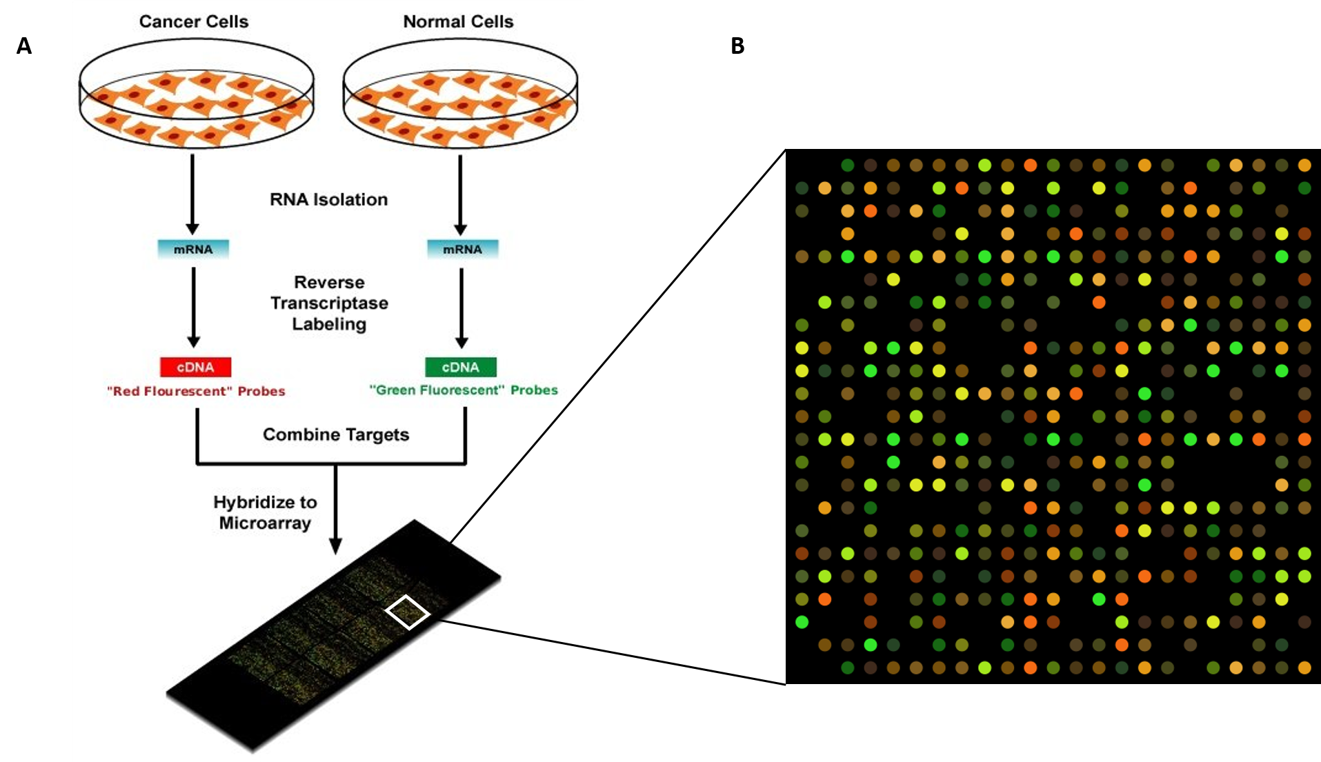
Figure \(\PageIndex{3}\): Diagram of a typical dual-color microarray experiment. Within a dual-color microarray, the probe DNA is typically hybridized with cDNA prepared from two different samples, each labeled with a different fluorescent probe. The analysis will yield green fluorescence from one sample that upregulates gene expression, whereas the other sample, tagged with a red fluorescence marker, will indicate that the other condition elicits gene expression at that location. Yellow indicates gene expression in both samples. Image A is modified from Larssono and Image B from Guillaume Paumier

Two-color microarrays, or two-channel microarrays, are typically hybridized with cDNA prepared from two samples to be compared (e.g., diseased tissue versus healthy tissue) and labeled with two different fluorophores. Fluorescent dyes commonly used for cDNA labeling include Cy3, which emits at 570 nm (green), and Cy5, which emits at 670 nm (red). The two Cy-labeled cDNA samples are mixed and hybridized to a single microarray, which is then scanned with a microarray scanner to visualize the fluorescence of the two fluorophores after excitation with a laser beam of a defined wavelength. The relative intensities of each fluorophore may then be used in a ratio-based analysis to identify up-regulated and down-regulated genes.

Oligonucleotide microarrays often carry control probes designed to hybridize with RNA spike-ins. The degree of hybridization between the spike-ins and the control probes is used to normalize the hybridization measurements for the target probes. Although absolute levels of gene expression can be determined in the two-color array in rare instances, relative differences in expression among spots within a sample and between samples are the preferred method of data analysis for the two-color system. Examples of providers for such microarrays include Agilent with their Dual-Mode platform, Eppendorf with their DualChip platform for colorimetric Silverquant labeling, and TeleChem International with Arrayit.

In single-channel microarrays or one-color microarrays, the arrays provide intensity data for each probe or probe set, indicating a relative level of hybridization with the labeled target. However, they do not truly indicate the abundance of a gene but rather a relative abundance compared to other samples or conditions processed in the same experiment. Each RNA molecule encounters protocol- and batch-specific biases during the experiment's amplification, labeling, and hybridization phases, rendering comparisons between genes on the same microarray uninformative. Comparing two conditions for the same gene requires two separate single-dye hybridizations. Several popular single-channel systems are the Affymetrix "Gene Chip", Illumina "Bead Chip", Agilent single-channel arrays, the Applied Microarrays "CodeLink" arrays, and the Eppendorf "DualChip & Silverquant". One strength of the single-dye system lies in the fact that an aberrant sample cannot affect the raw data derived from other samples because each array chip is exposed to only one sample (as opposed to a two-color system in which a single low-quality sample may drastically impinge on overall data precision even if the other sample was of high quality). Another benefit is that data can be more easily compared with arrays from different experiments, as long as batch effects have been accounted for.

Summary

(Summary written by Claude, Sonnet 4.6, Anthropic)

This chapter introduces DNA microarray technology as a tool for simultaneously measuring the expression levels of thousands to millions of genes across the genome in a single experiment, providing a powerful high-throughput platform for comparative gene expression profiling, genotyping, and functional genomics.

The fundamental principle of microarray technology is nucleic acid hybridization — the formation of Watson-Crick hydrogen bonds between complementary single-stranded nucleic acid sequences. Each microarray consists of a solid support (typically glass, silicon, or plastic) onto which thousands to millions of features are arranged in a precise grid, each feature containing picomolar quantities of a specific oligonucleotide probe sequence complementary to a transcript of interest. The experimental workflow begins with RNA extraction from cells or tissues under the conditions to be compared. The RNA is reverse-transcribed into cDNA using reverse transcriptase, and the resulting cDNA is fluorescently labeled (typically with Cy3 or Cy5 cyanine dyes). The labeled target is applied to the array under high-stringency hybridization conditions (controlled temperature, salt, and formamide concentration) that favor specific probe-target base pairing over non-specific interactions. After hybridization, the array is washed to remove unbound or weakly bound sequences, then scanned by a laser excitation system to measure fluorescence emission intensity at each feature. Because the identity of the probe at each feature is known by its spatial position on the array, the pattern of fluorescence intensities across the entire array constitutes a genome-wide snapshot of relative transcript abundance.

Microarray fabrication takes two principal forms. In spotted (contact-printed) arrays, pre-synthesized oligonucleotides, cDNA, or PCR products are deposited at defined positions on glass slides using robotic pin arrays that are dipped into individual probe solutions and then stamped onto the array surface. This approach is flexible and lower-cost, allowing investigators to customize the probe content for specific experiments, but reproducibility and sensitivity can be lower than those of commercial alternatives due to small batch sizes and variable printing efficiencies. In in situ-synthesized oligonucleotide arrays, probe sequences are built directly on the array surface one nucleotide at a time. Affymetrix GeneChips use photolithographic synthesis on silica wafers, where light-sensitive chemical protecting groups on each nucleotide precursor are selectively removed by UV illumination through photomasks (or dynamic micromirror arrays in maskless synthesis), allowing one nucleotide to be added to each exposed position per cycle; 25-mer probes are produced at very high density. Agilent arrays use ink-jet technology to synthesize 60-mer probes, providing higher per-probe specificity at the cost of slightly lower feature density. Longer probes (60-mers) provide greater hybridization specificity for individual transcript sequences, while shorter probes (25-mers) allow higher feature density and lower synthesis cost but may show more cross-hybridization.

Two-color (dual-channel) microarrays are the classic comparative format: cDNA from two experimental conditions (e.g., cancer cells vs. normal cells, drug-treated vs. untreated) is labeled with spectrally distinct fluorophores — Cy3 (excitation ~550 nm, emission ~570 nm, green) for one condition and Cy5 (excitation ~649 nm, emission ~670 nm, red) for the other — mixed in equal amounts, and co-hybridized to the same array. The scanner measures both fluorescence channels simultaneously at each feature, and the Cy5/Cy3 ratio at each spot provides a direct comparison of transcript abundance between the two conditions: green features indicate higher expression in the Cy3-labeled sample; red features indicate higher expression in the Cy5-labeled sample; yellow features (comparable Cy3 and Cy5 signals) indicate similar expression under both conditions. Ratio-based analysis normalizes for differences in probe binding efficiency across features and provides internally controlled comparisons, but a low-quality sample can compromise data from the paired channel. Single-color (single-channel) arrays expose each array to only one fluorescently labeled sample, measuring absolute signal intensity at each feature as a proxy for relative transcript abundance. While individual single-channel arrays cannot directly compare two conditions, multiple single-channel arrays from different samples can be compared statistically when appropriate normalization (using spike-in RNA controls of known concentration to calibrate signal intensities and correct for batch effects) is applied. The single-channel approach avoids cross-contamination between samples on the same chip and facilitates cross-experiment comparisons.

Data interpretation and applications require careful consideration of normalization and statistical analysis, since fluorescence intensity values reflect relative rather than absolute mRNA abundance and are subject to biases introduced at the amplification, labeling, and hybridization steps. Spike-in controls — known amounts of synthetic RNA sequences designed not to match any probe on the array — provide normalization standards by allowing measured signals to be calibrated against known input quantities. Computational analysis identifies differentially expressed genes by comparing normalized intensity ratios across conditions and applying statistical thresholds (e.g., fold-change cutoffs, false discovery rate corrections) to distinguish biologically meaningful from chance differences. Beyond gene expression profiling, microarray platforms are used for genotyping (single-nucleotide polymorphism arrays, comparative genomic hybridization to detect chromosomal copy number variations in cancer), splice variant detection (exon arrays with probes spanning individual exons), and ChIP-chip analysis (combining chromatin immunoprecipitation with microarray hybridization to map genome-wide protein-DNA interactions). Although microarrays have been largely supplemented by RNA sequencing (RNA-seq) in many applications — because RNA-seq provides absolute rather than relative transcript quantification, detects novel transcripts without prior probe design, and has a wider dynamic range — microarrays remain valuable for high-throughput, cost-effective analysis of well-characterized genomes and for specific clinical diagnostic applications where the gene targets are predetermined.