5.1: Binding - The First Step Towards Protein Function

Search Fundamentals of Biochemistry

Learning Goals 

(Learning goals written by Claude, Sonnet 4.6, Anthropic)

Equilibrium Binding: Mathematical Framework

• Define the dissociation constant K_D as the reciprocal of K_eq for the M + L ↔ ML equilibrium, explain why K_D is expressed in units of molarity and why biochemists prefer K_D over K_eq as the descriptor of binding strength, and use the operational definition of K_D — the free ligand concentration at half-maximal macromolecule saturation — to rapidly estimate binding extent from a graph.
• Derive and apply the two fundamental binding equations: Y = L/(K_D + L) for the case where L ≈ L₀ (excess ligand), and the quadratic equation for ML as a function of M₀, L₀, and K_D for the general case — recognizing when each is appropriate and understanding that both give the same ML at a given set of conditions.
• Interpret hyperbolic (Y vs. L), semi-logarithmic (Y vs. log L), double-reciprocal (1/Y vs. 1/L), and Scatchard (Y/L vs. Y) plots of binding data — identifying K_D and binding site number from each graphical form, explaining why nonlinear fitting of hyperbolic data is statistically superior to linear transformations, and distinguishing true sigmoidal binding (cooperative, allosteric) from the sigmoidal appearance of semilog plots of simple hyperbolic binding.

Binding Kinetics, Affinity, and the Binding Continuum

• Relate K_D to the microscopic rate constants for association and dissociation (K_D = k_off/k_on), calculate k_off and the half-life of a protein-ligand complex given K_D and an assumed diffusion-limited k_on (~10⁸ M⁻¹s⁻¹), and use the resulting table of t½ values to develop intuition for how K_D values spanning picomolar to millimolar translate into complex lifetimes spanning years to microseconds.
• Place a given binding interaction on the binding continuum from no interaction (ΔG° ≈ +100 kcal/mol, K_D ≈ 10⁷³ M) to covalent bond formation (ΔG° ≈ −97 kcal/mol), use the relationship ΔG° = −RT ln K_eq = RT ln K_D to interconvert between KD, Keq, and ΔG°, and distinguish specific from nonspecific binding in terms of structural complementarity, biological context, and KD magnitude.
• Derive the binding equation for protein dimerization (M + M ↔ M₂) using mass balance for a self-associating system, explain why fractional dimer formation at M₀ = K_D is not equivalent to half-maximal saturation in the simple M + L ↔ ML case, and describe the biological implications of protein concentration relative to K_D for determining the physiologically relevant aggregation state.

Modulators of Ligand-Protein Interactions

• Explain the LOCKTAC (load and lock targeting chimera) concept — drugs that bind outside the orthosteric site and alter koff of an endogenous ligand rather than competing for the binding site — distinguishing activator LOCKTACs (which extend complex lifetime when the bound state is active) from inhibitory LOCKTACs (which extend complex lifetime when the bound state is inactive), using risdiplam, peloruside, sovilnesib, and trametinib as examples.

Reversible Binding of a Ligand to a Macromolecule

Reversible, noncovalent binding of two or more molecules is the first step in expressing the biological properties of almost all biomacromolecules. If one of the molecules is small, it's often called a ligand. Ligands are often called other names. Substrates are the reactants that bind to the active sites of enzymes. Hormones and neurotransmitters bind to solution-phase or membrane-bound receptor proteins. Metal ions (e.g., monatomic divalent cations like Ca²⁺, or molecular, like CH₃CO₂^-) are also considered ligands when bound to proteins or nucleic acids.

You might be more familiar with the term ligand when it's applied to the coordination of a transition metal complex by electron pair donors (Lewis acids) on single or multidentate molecules, which for transition metal complexes are called ligands. Here is an interactive molecule model of a cobalt ion binding to EDTA, a multidentate ligand.

The cobalt ion (dark grey ball) is octahedrally coordinated to the multidentate ligand EDTA.

Whether a macromolecule M and a ligand L bind to each other depends on their relative concentrations and how tightly they bind. Compare this to an acid. Its pKa and the pH of the medium determine if it deprotonates.

Biochemists rarely discuss equilibrium constants to describe the strength of a binding interaction, but rather their reciprocals - the dissociation constants, \(K_D\). For the reactions \(M + L ↔ ML\), where M is a free macromolecule, L is a free ligand, and ML is a macromolecule-ligand complex (which is held together by intermolecular forces, not covalent forces), the K_D is given by

\begin{equation}
\left.K_D=[M]_{e q}\right][L]_{e q} /[M L]_{e q}
\end{equation}

Figure \(\PageIndex{1}\) shows free and bound M and L.

Figure \(\PageIndex{1}\): Free macromolecule (M), free ligand (red triangle) and bound complex ML

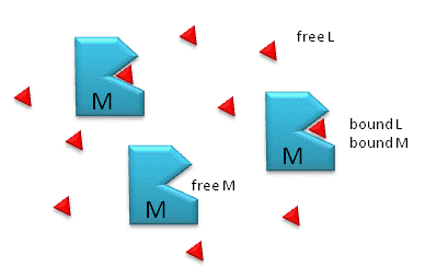
Notice the unit of K_D is molarity, M.

• The lower the K_D (i.e., the higher the [ML] at any given M and L), the tighter the binding.
• The higher the K_D, the looser the binding. K_Ds for biological molecules are finely tuned to their environments.

KD values vary from about 1 mM (weak interactions) for some enzyme-substrate complexes to pM-fM levels. Examples of very tight, non-covalent interactions include the avidin (an egg protein)-biotin (a vitamin) and thrombin (enzyme initiating clotting)-hirudin (a leech salivary protein) complexes. The values are "tuned" so that the relative concentrations of free and bound M and L are appropriate for a biological setting.

To understand binding, it is important not only to know the non-covalent interactions that lead to binding but also to ask the simple question: Is the ligand bound to the macromolecule? If so, to what extent? To know if M or L is bound, we must use simple mathematics that you would have learned in Introductory or Analytical Chemistry courses. We'll start with the mathematical description, which students are likely to find less intuitive than that of noncovalent interactions.

We will start with three basic equations:

For the Dissociation constant:

\begin{equation}
K_D=([M] e q[L] e q) /[M L] e q=([M][L]) /[M L]
\end{equation}

(Note that K_D has units of molarity.);

For Mass Balance of M:

\begin{equation}
M_0=M+M L
\end{equation}

where M₀ is the total amount of macromolecule. (note: brackets and the eq subscript will be left off if the resulting equation is non-ambiguous)

For Mass Balance of L:

\begin{equation}
L_0=L+M L
\end{equation}

where L₀ is the total amount of ligand

We want to derive equations that give ML as a function of known or measurable values. The K_D equation (5.1) shows that ML depends on free M and free L. From the equations above, we can derive two fundamental and equally valid equations that are useful under different experimental conditions.

Case 1:

This applies when you can readily measure free L OR when experimental conditions are that Lo >> Mo (so L= Lo), often encountered in a lab setting. You don't have to measure free L, since in this case it is approximately equal to the total ligand added to the system.

Substitute 5.1.3 into 5.1.1 gives

\begin{equation}
\begin{gathered}
\left.K_D=([M][L]) /[M L]=[M o-M L][L]\right) /[M L \\
(M L) K_D=\left(M_o\right) L-(M L) L \\
(M L) K_D+(M L) L=\left(M_o\right) L \\
(M L)\left(K_D+L\right)=\left(M_0\right) L
\end{gathered}
\end{equation}

or

\begin{equation}
(M L)=\frac{\left(M_0\right) L}{K_D+L}
\end{equation}

This equation is ALWAYS TRUE for the chemical equation written above. L is the free ligand concentration at equilibrium.

An interactive plot of the concentration of the ML complex (ML) vs free L (L) is shown below. Vary the sliders and note the changes in the graph.

If L₀ >> M₀, then the equations simplify to:

\begin{equation}
M L=\frac{\left(M_0\right)\left(L_0\right)}{K_D+L}
\end{equation}

Dividing this equation by Mo gives the fractional saturation Y of the macromolecule M.

\begin{equation}
Y=[M L] / M_0=\frac{L}{K_D+L}
\end{equation}

where Y can vary from 0 (when L = 0) to 1 (when L >> K_D)

Note that the interactive graph above and graphs of ML vs L (equation 5.1.10) and Y vs L (equation 5.1.11) are all HYPERBOLAS

To get a "gut" level understanding of the graphs of \((ML) = (M_0)(L)/(K_D + L)\) and \(Y = L/(K_D+L)\), let's consider 3 different values or sets of values of free ligand:

1. L = 0: This gives ML = 0
2. L = K_D: \((ML) = (M_0)(L)/(L + L)= (M_0)(L)/(2L) = Mo/2\) which indicates that M is half saturated. The operational definition of K_D is the ligand concentration at which the M is half-saturated.
3. L >> K_D: ML = M₀, and the macromolecule is saturated with ligand.

Case 2 (more general):

This applies when you know K_D, but don't know free L or haven't measured it, and you wish to calculate how much ML is present at equilibrium, given a K_D value. L₀ does not have to be much greater than M₀ in this case. If it were, like it is often in an experimental system, you would know that free L = L₀, and you could use Case 1.

In this case, we will substitute mass balance equations for both M₀ (Eq 5.1.2) and L₀ (Eq 5.1.3) into the equation for K_D (Eq. 5.1.1). This gives:

\begin{equation}
\begin{gathered}
K_D=([M][L]) /[M L]=\left[M_0-M L\right]\left[L_0-M L\right] /[M L] \\
(M L) K_D=\left(M_0-M L\right)\left(L_0-M L\right) \\
(M L) K_D=\left(M_0\right)\left(L_0\right)-(M L)\left(L_0\right)-(M L)\left(M_0\right)+(M L)^2
\end{gathered}
\end{equation}

or

\begin{equation}
(M L)^2-\left(L_0+M_0+K_D\right)(M L)+\left(M_0\right)\left(L_0\right)=0
\end{equation}

This can be rearranged into the form \(ax^2 + bx + c = 0\) where

• a = 1
• b = - (L₀ + M₀ +K_D)
• c = (M₀)(L₀)

with the well known solution \(x = [(-b) - (b^2 - 4(a)(c))^{1/2}]/2a\). Therefore,

\begin{equation}
(M L)=\left[\left(L_0+M_0+K_D\right)-\left(\left(L_0+M_0+K_D\right)^2-4\left(M_0\right)\left(L_0\right)\right)^{1 / 2}\right] / 2
\end{equation}

An interactive plot of Y, the fractional saturation, vs. total L (L₀) is shown below. Vary the sliders and note the changes in the graph.

In the derivations, we derived two equations for ML: Eq 5.1.10, which gives ML vs. L, and Eq 5.1.16, which gives ML vs. L_0.

Both equations are valid. In the first, you must know free L, which is often L₀ if M₀ << L₀. In the second, you don't need to know free M or L at all. At a given Lo, Mo, and K_D, you can calculate ML, which should be the same ML you get from the first equation if you know free L.

Equations 5.1.10 and 5.1.16 are useful in several circumstances. They can be used to

• calculate the concentration of ML if K_D, M₀, and L (for Eq. 5.1.10) or if K_D, M₀, and L₀ (for Eq. 5.1.16) are known. This is analogous to using the Henderson-Hasselbalch equation to calculate the protonation state (HA) and, hence, the acid's charge state at various pH values. In the former binding case, we measure the concentration of a reversibly bound ligand (ML), and in the latter case, we measure the concentration of covalently bound protons (HA).
• calculate K_D if ML, M₀, and L (for Eq. 5.1.10) or if ML, M₀, and L₀ (for Eq. 5.1.16) are known. A separate chapter will discuss techniques for extracting the K_D from binding data.

Interpretation of Binding Analyses

It is important to get a mathematical understanding of the binding equations and graphs. It is equally important to get an intuitive understanding of their properties. Just as we used the +/- 2 pH rule to determine at a glance the charge state of an acid, you need to be able to determine the extent of binding (how much of M is bound to L) given their relative concentrations and the K_D. The usual situation is that [M₀] is << [L₀]. What happens to the binding curves for M + L ↔ ML if the K_D gets progressively lower? Intuitively, you should expect binding to increase, especially as L increases. The curves below should help you develop the intuition you need with respect to binding equilibria. Figure \(\PageIndex{2}\) show Y vs L₀ at Varying K_Ds.

Figure \(\PageIndex{2}\): Fractional saturation Y vs L₀ at Varying K_Ds

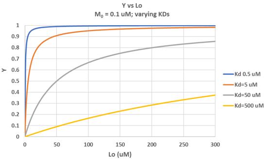
Figure \(\PageIndex{3}\) shows Y vs L₀ at a very low K_D (0.001 uM = 1 nM, resulting in a sharp "titration" curve. Any increment of L added is bound, so effectively, none is present in the free form. The graph abruptly changes to a horizontal line when all the macromolecules are bound. This curve could be used to determine [M₀]!

Figure \(\PageIndex{3}\): Fractional saturation Y vs L₀ for very low K_D binding interactions

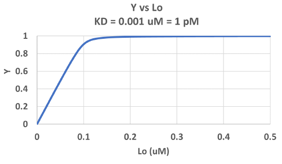
Note that in the last graph, given the same M₀ and L₀ concentrations, the "titration curves" for a binding equilibrium characterized by even tighter binding (for example, a K_D = 0.1 pM or 0.01 pM) would be indistinguishable from the graph when K_D = 1 pM. It should be apparent that for all of these K_D values, all of the added ligand is bound until [L₀] > [M₀]. To differentiate these cases, much lower ligand concentrations would be required so that all is not bound upon the addition of ligand. Also note that this curve is NOT hyperbolic, which makes sense since the graph is of Y vs L₀, not Y vs L, and since L₀ is not >> M₀.

The interactive graph below shows fractional saturation Y vs L at two different K_D values

It is quite interesting to compare graphs of Y (fractional saturation) vs L (free) and Y vs Lo (total L) in the special case when L₀ is not >> M₀. Figure \(\PageIndex{4}\) when M₀ = 4 μM, Kd = 0.19 μM . Under the ligand concentration used, it should be apparent that L can't be approximated by L₀

Figure \(\PageIndex{4}\): Fractional saturation Y vs L or L₀ when L₀ is not >> M₀

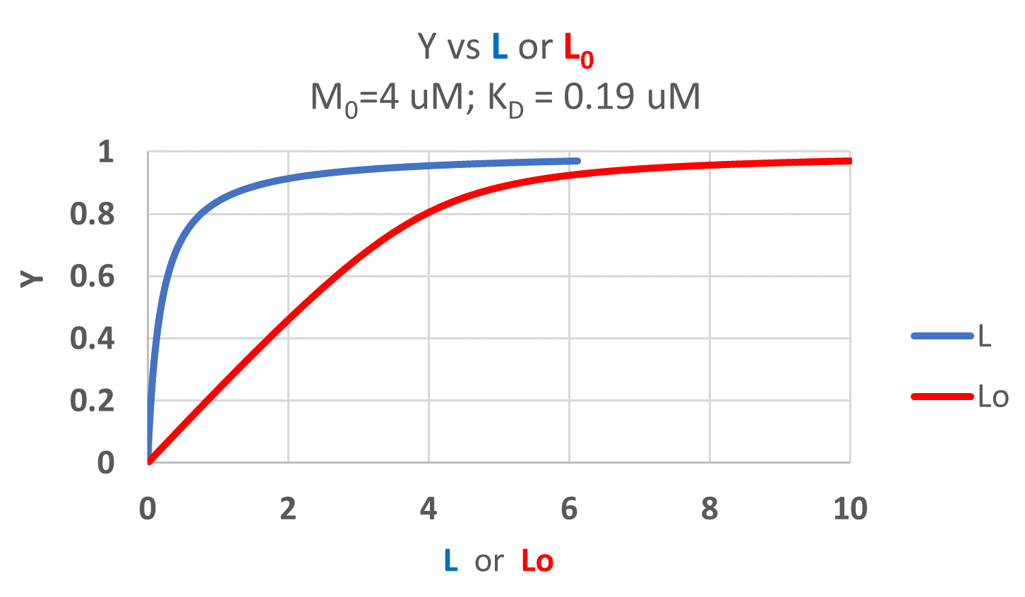
Two points should be evident from these graphs when L is not approximated by Lo:

• a graph of Y vs L₀ is not truly hyperbolic, but it does saturate
• a K_D value (ligand concentration at half-maximal binding) can not be estimated by inspection from the Y vs L₀, but it can be from the Y vs. L graph.

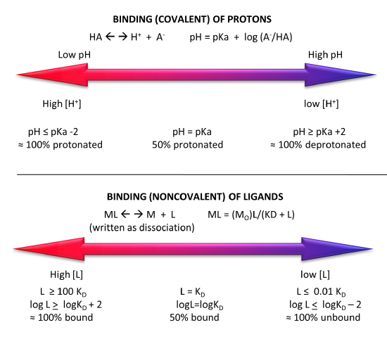
Figure \(\PageIndex{5}\) shows a comparison of the extent of covalent binding of a proton to an acid at pH values around the pKa and, by analogy, the extent of noncovalent binding of a ligand at log[L] values around the log K_D.

Figure \(\PageIndex{5}\): Analogy between covalent binding of protons and noncovalent binding of ligands to a molecule

Different Graphical Analyses of Binding

In addition to the hyperbolic plots of [ML] vs [L] and fractional saturation Y vs [L], a variety of derivative plots are often encountered. The equations and their graphs (for two different K_D values) are shown below. The graphs are in the form of Y vs. L₀, where L₀ is approximately equal to the free L.

Hyperbolic saturation plot:

\begin{equation}
\mathrm{Y}=\frac{\mathrm{L}}{\mathrm{K}_{\mathrm{D}}+\mathrm{L}}
\end{equation}

Double reciprocal plot:

\begin{equation}
\frac{1}{\mathrm{Y}}=\frac{\mathrm{K}_{\mathrm{D}}+\mathrm{L}}{\mathrm{L}}=\frac{\mathrm{K}_{\mathrm{D}}}{\mathrm{L}}+1=\mathrm{K}_{\mathrm{D}}\left(\frac{1}{\mathrm{~L}}\right)+1
\end{equation}

A plot of 1/Y vs 1/L has a slope of K_D and a y-intercept of 1 (which is the number of binding sites for this simple mechanism)

The Scatchard plot:

\begin{equation}
\begin{aligned}
\mathrm{Y}\left(\mathrm{K}_{\mathrm{D}}+\mathrm{L}\right) &=\mathrm{L} \\
Y\left(\mathrm{~K}_{\mathrm{D}}\right)+Y L &=L \\
Y\left(\mathrm{~K}_{\mathrm{D}}\right)=L-\mathrm{YL} &=\mathrm{L}(1-\mathrm{Y})
\end{aligned}
\end{equation}

which gives the final Scatchard plot equation:

\begin{equation}
\frac{Y}{\mathrm{~L}}=\frac{1-\mathrm{Y}}{\mathrm{K}_{\mathrm{D}}}=-\frac{\mathrm{Y}}{\mathrm{K}_{\mathrm{D}}}+\frac{1}{\mathrm{~K}_{\mathrm{D}}}
\end{equation}

A plot of Y/L vs Y has a slope of -1/K_D and a y-intercept of 1/K_D.

Y vs logL

Plotting Y vs L yields a hyperbola, whereas plotting Y vs log L yields a sigmoidal curve. Plots of Y vs log L are often used in the research literature instead of traditional hyperbolic plots of Y vs L. There are several reasons for this:

• The log [L] is more fundamentally related to the thermodynamic expression that relates ΔG⁰ and K_eq or K_D, namely

\begin{equation}
\Delta G^0=-R T \ln K_{e q}=R \operatorname{Tln} K_D
\end{equation}

• plots of Y vs. L plateau over a very large range of [L], but given the compression of the X-axis values in a semilog plot, the plots reach a saturation plateau over a much narrower range of log [L]. A range from 1-100 on the [L] scale becomes 0-2 on the log [L] scale. Since it takes a very high ligand concentration to reach true saturation (100xK_D), it's much easier to see whether saturation is achieved in semilog plots.
• multiple plots of binding data for different K_D values have the same shape on a semilog plot. Binding data for a ligand to wild-type and mutant proteins, each with different K_Ds, will yield identical plots, with curves for higher K_D values shifted to the right. Semilog plots are also routinely used to display multiple binding curves in the absence and presence of a binding inhibitor.

Figure \(\PageIndex{6}\) show different graphs for ligand binding to a macromolecule

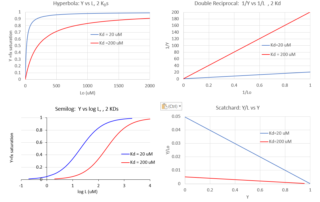
Figure \(\PageIndex{6}\): Different graphs for ligand binding to a macromolecule

Sigmoidal binding curves: A note of caution

The graph of Y vs. log [L] is sigmoidal, but the same data would give a hyperbola if plotted as Y vs. [L]. However, as we will see in section 5.3, there are some occasions when the graph of Y vs. [L] is sigmoidal. For example, this can occur when the binding of a ligand to a multimeric binding protein affects its binding to additional sites on the protein. This is an example of allosteric binding, which we will explore in detail in section 5.3. So, if you see a sigmoidal plot, be careful to examine the graph to see if it is a regular or semilog plot.

Straight line transformations of the hyperbolic binding equations are useful to get approximate values of K_D, but linear regression analysis to get slopes and intercepts is not statistically optimal, as the errors in the y variable (Y) and the y and x variables in the Scatchard plot are not identical across values. To determine K_D, it is best to fit the experimental data to the hyperbolic function.

Dimerization and Multiple Binding Sites

In the previous examples, we considered the case of a macromolecule M binding a ligand L at a single site, as described in the equation below:

M + L ↔ ML

where K_D = [M][L]/[ML]

We saw that the binding curves (ML vs L or Y vs L are hyperbolic, with a K_D = L at half-maximal binding. But many other chemical equilibria can mechanistically explain binding data. We'll consider just two cases here.

Dimerization

A special yet common example of this equilibrium occurs when a macromolecule binds itself to form a dimer (D), as shown below:

M + M ↔ M₂ or D

where D is the dimer, and where

\begin{equation}
K_D=[M][M] /[D]=[M]^2 /[D]
\end{equation}

At first glance, you would expect a graph of [D] vs [M] to be hyperbolic, with the K_D again equaling the [M] at half-maximal dimer concentration. This turns out to be true, but a simple derivation is in order. In the case of dimer formation, Mo, which superficially represents both M and L in the earlier derived expression, is changing. So we have to invoke mass balance of M again: \([Mo] = [M] + 2[D]\), where the coefficient 2 is necessary since there are 2 M in each dimer.

More generally, for the case of the formation of trimers (Tri), tetramers (Tetra), and other oligomers, \([Mo] = [M] + 2[D] + 3[Tri] + 4[Tetra] + ....\)

Rearranging (12) and solving for D gives \(D = ([M_0] - [M])/2\). Substituting this into the K_D expression (1) gives

\begin{equation}
K_D=\frac{M^2}{\frac{\left[M_0\right]-[M]}{2}}=\frac{2 M^2}{\left[M_0\right]-[M]}=
\end{equation}

This can be rearranged into quadratic form for M (not D):

\begin{equation}
2 M^2+K_D(M)-K_D\left(M_0\right)=0
\end{equation}

which is of the form y = ax²+bx+c.

Solving the quadratic equation gives [M] and with M₀ , D can be calculated from \(D = ([M_0]-[M])/2\).

A value Y, similar to fractional saturation, can be calculated, where Y is the fraction of total possible D, which can vary from 0 to 1: \(Y= 2D/M_0\)

A graph of Y vs Mo with a dimerization dissociation constant K_D = 25 uM is shown in Figure \(\PageIndex{7}\).

Figure \(\PageIndex{7}\): Fractional saturation Y vs M₀ for protein dimerization

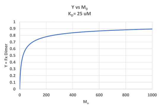
Note that the curve appears somewhat hyperbolic. Half-maximal dimer formation does occur at a total M concentration M₀ = K_D. Also note, however, that even at M₀ = 1000 uM, which is 40x K_D, only 90% of the total possible D is formed (Y = 0.90). For the simple M + L ↔ ML equilibrium, if L₀ = 40x the K_D and M₀ << L₀, \(Y = L/(K_D+L) = L/[(L/40)+L] = 0.976\)

An interactive graph showing Y (the fraction of dimers) vs M₀ is shown. Move the sliders to show how changes in "K_D" affect the dimerization.

The aggregation state of a protein monomer is closely linked to its biological activity. Some proteins that can form dimers are active in the monomeric state, while others are active as dimers. High concentrations, as encountered during protein crystallization for X-ray structure analysis, can drive proteins into the dimeric state. This may lead to the false conclusion that the active protein is a dimer. Determination of the actual physiological concentration of [Mo] and K_D provides investigators with the Y value, which can be correlated with biological activity. For example, interleukin 8, a chemokine that binds certain immune cells, exists as a dimer in X-ray and NMR structural determinations but as a monomer at physiological concentrations. Hence, the monomer, not the dimer, binds its receptors on immune cells. Viral proteases (herpes viral protease, HIV protease) are active as dimers, with the active site located at the dimer interface.

Binding of a ligand to two independent sites

What if a ligand L binds to two different sites on the same biomacromolecule? Assuming that the binding of ligand L to one site does not affect the binding of the ligand to the other site (and vice versa), the following equation can be derived:

\begin{equation}
Y=\left[\frac{L}{\left(K_{D 1}+L\right)}+\frac{L}{\left(K_{D 2}+L\right)}\right] / 2
\end{equation}

The numerator of the equation has a term for the fractional saturation of site 1 characterized by K_D1 and a term for the fractional saturation of site 2 characterized by K_D2. These two terms are divided by 2 so that the fractional saturation of all sites is 1 at saturating values of free ligand. Note that there can only be one free ligand concentration in solution, so the difference in the two terms in the numerator is the K_D value.

The interactive graph below shows such binding to two independent sites with different K_D values. Again, we'll assume the binding of one ligand does NOT influence the binding of the other.

The Binding Continuum

Binding affinities allow us to measure the relative strength of binding between two substances. But how "tight" is tight binding? Weak binding? Let us examine that issue by considering a binding continuum. Consider two substances, A and B, that might interact. Over what range of strengths can they actually bind to each other? It would be helpful to set up the extremes of the binding continuum. At one end, there is no binding at all. At the other end, consider two things that bind covalently. We have discussed how Kd reflects binding strength. Remember, K_D = 1/K_eq. Also, we know that K_eq is related to ΔG^o by the equations:

\begin{equation}
\Delta G^0=-R \operatorname{Tln} K_{e q}=R \operatorname{Tln} K_D
\end{equation}

Given these simple equations, you should be able to interconvert between K_eq, K_D, and ΔG⁰. (Keep your units straight.)

No interaction: One end of the binding continuum represents no interaction. Let's assume that K_eq is tiny (K_D large) - for example, K_eq ~ 2.4 x10^-72. Plugging this into the equation \(ΔG^0 = - RTlnK_{eq}\), where R = 2.00 cal/mol^.K, and T is about 300K, the ΔG⁰ ~ +100 kcal/mol (418 kJ/mo). If we add A + B, there is no drive to form AB. If AB did form, then it would immediately fall apart.

Covalent interaction: At the other end of the continuum, consider the interaction of 1H atom with another to form H₂. From a general chemistry book, we can get ΔG⁰ _form . Using simple thermodynamics, we can calculate ΔG^o for H-H formation. (ΔG^o = ΣΔG⁰ _form prod. - ΣΔG⁰ _form react.) Doing this gives  -97 kcal/mol (-406 kJ/mol).

Specific and Nonspecific Binding: Consider the interaction between the lambda repressor (R) and a small oligonucleotide to which it binds tightly (the operator DNA, O). This is an example of a biologically tight but reversible interaction. Due to electrostatic interactions and H bonds between the positively charged protein and the negatively charged nucleic acid backbone, R can bind to many short oligonucleotides. The tight-binding interaction, however, involves oligonucleotides with a specific base sequence. Hence, we can distinguish between tight binding, which usually involves specific DNA sequences, and weak binding, which involves nonspecific sequences. Likewise, we will speak of specific and nonspecific binding. R and O, which bind with a K_D of 1 pM, represent an example of specific binding.

In contrast, R and nonspecific DNA (D), which bind primarily through electrostatic interactions with a K_D of 1 mM, are examples of nonspecific binding. You might expect any positively charged protein, like mitochondrial cytochrome C, would bind negatively charged DNA. This nonspecific interaction would presumably have no biological significance since the two are localized in different cell compartments. In contrast, the interaction between positively charged histone proteins bound to DNA in the nucleus would be specific.

Rate constants for association and dissociation: When the reaction
M + L ↔ ML is at equilibrium, and the forward reaction rate is equal to the reverse reaction rate. As you learned in introductory chemistry, the forward reaction is bimolecular and second-order. Hence, the v_f, the rate in the forward direction, is proportional to [M][L] or
\(v_f = k_f[M][L]\), where k_f is the rate constant in the forward direction. The rate of the reverse reaction, v_r is first order, proportional to [ML], and is given by \(v_r = k_r [ML]\), where k_r is the rate constant for the reverse reaction. Notice that the units of k_f are M^-1s^-1, while the units of k_r are s^-1. At equilibrium, \(v_f = v_r\), or

\begin{equation}
k_f[M][L]=k_r[M L]
\end{equation}

Rearranging the equation gives

\begin{equation}
[M L] /[M][L]=k_f / k_r=K_{e q}
\end{equation}

Hence, K_eq is given by the ratio of rate constants. For tight binding interactions, K_eq >> 1, K_D << 1, and k_f is very large (in the order of 10^8-9 ), and k_r must be very small (10^-2 - 10 ^-4 s^-1).

To get a more intuitive understanding of K_Ds, it is often easier to think about the rate constants that contribute to binding and dissociation. Let us assume that k_r is the rate constant that describes the dissociation reaction. It is often called k_off. Likewise, k_f is often called the on rate (k_on). It can be shown mathematically that the rate at which two simple molecules associate depends on their radius and effective molecular weight. The maximal rate at which they will associate is the maximal rate at which diffusion will lead them together. Let us assume that the rate at which M and L associate is diffusion-limited. The theoretical k_on is about 10⁸ M^-1s^-1. Knowing the K_D and that k_on/k_off = K_eq = 1/K_D, we can calculate k_off, the first-order rate constant.

We can also determine k_off experimentally. Imagine the following example. Adjust the concentrations of M and L such that Mo << Lo and Lo>> Kd. Under these conditions of ligand excess, M is entirely in the bound form ML. Now, at t = 0, dilute the solution so that Lo << Kd. The only process here is dissociation, since negligible association can occur given the new condition. If you can measure the biological activity of ML, you can measure the rate of ML disappearance over time and obtain k_off. Alternatively, if you could measure M's biological activity, the rate at which activity returns will give you k_off.

You will remember from Introductory Chemistry that for a first-order rate constant, the half-life (t_1/2) of the reaction can be calculated by the expression k = 0.693/t_1/2. Hence, given k_off, you can determine the t_1/2 for the associated species'  existence. How long will a complex of ML last before it dissociates? Given ΔG^o or K_D, and assuming a k_on (10⁸ M^-1s^-1), you should be able to calculate k_off and t_1/2. Or, you could determine k_off experimentally and then calculate t_1/2. Applying these principles, you can calculate the binding parameters. Table \(\PageIndex{1}\) below shows calculated k_off and t_1/2 for binary complexes assuming diffusion-controlled k_on.

Complex	KD (M)	koff (s^-1)	t½
H2	1 x 10^-71	1 x 10^-63	2 x 10^55 yr
RtV3 : Rt'L3(a)	10^-17	1 x 10^-9	2 yr
Avidin:biotin	10^-15	1 x 10^-7	80 days
thrombin:hirudin(b)	5 x10^-14	5 x 10-6	2 days
lacrep:DNAoper(c)	1 x 10^-13	1 x 10^-5	0.8 days
Zif268:DNA(d)	10^-11	1 x 10^-3	700 s
GroEL:r-lactalbumin(e)	10^-9	0.1	7 s
TBP:TATA(f)	2 x 10^-9	2 x 10-1	3 s
TBP:TBP	4 x 10^-9	4 x 10^-1	2 s
LDH (pig): NADH(g)	7.1x10^-7(j)	7.1 x 10^1	10 ms
profilin: CaATP-G-actin	1.2 x 10-6	1.2 x 10^2	6 ms
TBP: DNAnonspec(h)	5 x 10^-6	5 x 10^2	1 ms
TCR(i): cyto C peptide	7X10^-5	7X10^3	100 us
lacrep:DNAnonspec(h)	1 x 10^-4	1 X10^4	70 us
uridine-3P: RNase	1.4x10^-4 (j)	1.4X104	50 us
Creatine Kinase: ADP	8.2x10-4 (j)	8.2X10^4	10 us
Acetylcholine:Esterase	1.2 x 10^-3	1.2 x 10^5	6 us
no interaction	4 x 10^73	4 x 10^81	-

Table \(\PageIndex{1}\): Calculated k_off and t_1/2 for binary complexes assuming diffusion-controlled k_on

1. Trivalent Vancomycin derivative RtV3 + Trivalent D-Ala-D-Ala deriv, Rt'L3'
2. Hirudin is a potent thrombin inhibitor from leech saliva
3. lac rep is the E. Coli lac operon repressor protein, and DNAoper is the specific DNA-binding region in the E. Coli genome that binds to the repressor
4. Zif268 is a mouse zinc-finger binding protein
5. GroEL is a chaperone protein; r-lactalbumin is the reduced form of lactalbumin
6. TBP is the TATA Binding Protein that binds to the TATA box consensus sequence
7. LDH is lactate dehydrogenase
8. DNA_nonspec is DNA that does not contain the specific DNA sequence region involved in a specific
   binding to a DNA-binding protein
9. TCR is the T-cell receptor
10. calculated from equation: KD = k_off/k_on.

What is usually measured is K_D and/or k_off (if the k_off is reasonable). This analysis is very simplified. Electrostatic forces and other orientation factors may significantly change k_on, while conformational changes in the complex may prevent ready unbinding of the bound ligand, dramatically altering k_off.

Figure \(\PageIndex{8}\) shows an interactive iCn3D model of one of the tightest binding complexes, avidin and biotin (2avi).

​

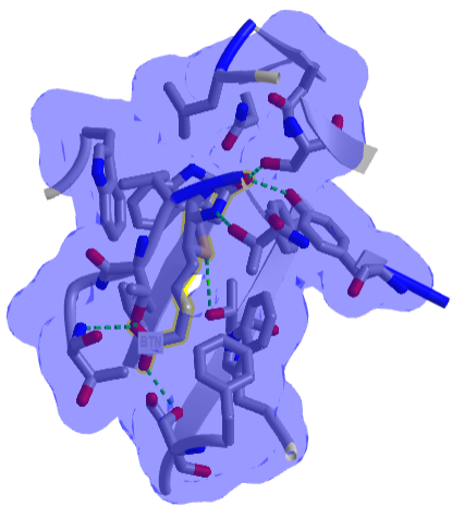
Figure \(\PageIndex{8}\): Avidin-Biotin Complex (2avi) (Copyright; author via source).
Click the image for a popup or use this external link: https://structure.ncbi.nlm.nih.gov/i...ZssSe5GoUfr9Q6

The blue indicates the surface around the complex, suggesting that the avidin is completely buried. Hydrogen bonds are shown to biotin (labeled as BTN) in green dashes.

It is important to note that even reactions characterized by high K_D (weak binding) can be specific. Specificity is ultimately defined as a binding interaction between a macromolecule and a ligand that can be co-localized in the same environment and for which a biological function is elaborated upon binding.

Recently added:  9/18/25

Modulators of Enzyme-Ligand Dissociation

Most medical drugs are designed to prevent the binding of a biological ligand to a target protein.  The drug often has a structure similar to an endogenous ligand, so both bind to the same site on the protein. It hence decreases the amount of ligand bound to the protein.  As mentioned above, it's important that once bound, a ligand or drug dissociates from the protein so that it is not permanently bound, which would leave the system in an unregulated state.  When binding to the same site as an endogenous ligand, the drug acts as a "competitive" inhibitor, decreasing the "effective" k_on for the endogenous ligand.  The drugs are designed to have a structure similar to the biological ligand or to be a complementary fit to the drug-binding site on the protein.  But what if the protein lacks a well-defined binding site or pocket?  How could you find or design a drug to affect the function of a protein? 

An alternative approach would be equally effective: design a drug that binds elsewhere on a protein but alters the k_off of a bound ligand.  This new drug could keep a protein:ligand complex bound longer than normal, by decreasing the effective k_off for the bound ligand. These new types of drugs have been called LOCKTACs, or “load and lock targeting chimeras”.  These drugs "lock together" the protein-ligand complex or promote its dissociation.  That name is similar to another type of "drug" called PROTACs (Proteolysis-Targeting Chimeras), which modify a protein, leading to its proteolysis and loss of the protein's function.  

By slowing the dissociation of the ligand, these LOCKTACs could alter the function of the protein in two ways.

• If the bound complex is active, the drug (an activator, LOCKTAC) could enhance or activate the protein's activity by keeping the ligand bound longer.  
• If the bound complex is inactive, the drug (an inhibitory LOCKTAC) could inhibit the protein's activity by keeping the ligand bound longer.

Here are two examples of activator LOCKTACs.

• Risdiplam: This drug stabilizes the interaction between SMN2 RNA and a splice factor, promoting better inclusion of exon 7 during splicing of the SMN2 gene transcript, which encodes the Survival Motor Neuron protein (SMN2), critical for motor neurons that control muscle movement. 
• Peloruside:  This drug enhances interactions between two proteins (β-catenin with a ligase) and also stabilizes tubulin polymers against dissociation (depolymerization).  

Figure \(\PageIndex{9}\) shows an interactive iCn3D models of the Tubulin-Peloruside A complex (4O4J).  Peloruside A, an activator LOCKTAC, promotes microtubule (MT) assembly by interacting at the interface between protofilaments and decreasing mobility, both of which maintain function.  

Figure \(\PageIndex{9}\): Tubulin-Peloruside A complex (4O4J).   (Copyright; author via source).
Click the image for a popup or use this external link: https://www.ncbi.nlm.nih.gov/Structu...820c7acf44b5dd

The tubulin monomers are shown in magenta, blue, brown, and green.  Two Peloruside A molecules are shown in spacefill.

Here are two examples of inhibitory LOCKTACs (that inhibit function by preventing dissociation).

• Sovilnesib: This drug traps the kinesin motor KIF18A protein on microtubules, preventing it from moving along the microtubules.  

• Trametinib:  This drug acts to inhibit the activity of the enzyme MEK and a complex of the enzyme, MEK:KSR, where KSR is a "scaffold" protein that presents MEK to a signaling pathway critical for cell growth.  This enzyme (a MAP Kinase) is hyperactive in many cancers.  It is a protein kinase that uses a bound ATP to phosphorylate and activate downstream proteins in its signaling pathway.  An upstream kinase must first phosphorylate MEK before it can phosphorylate other enzymes downstream in the pathway.  Trametinib binds at a different (allosteric) site than ATP, so it does not compete with ATP for its binding site, even if ATP levels are high.  Trametinib locks MEK in an inactive conformation even as it remains associated with KSR, but does not block MEK:KSR binding.  Hence, MEK is locked into an inhibitory form that can not be activated by upstream phosphorylation.

Figure \(\PageIndex{10}\) shows an interactive iCn3D model of the KSR2:MEK1 in complex with AMP-PNP (a non-hydrolyzable ATP analog), and the allosteric MEK inhibitor, Trametinib (7JUR).   KSR2 is in magenta and MEKI is in cyan.  The ATP analog is shown in sticks, and Trametinib is in spacefill.

Figure \(\PageIndex{10}\): KSR2:MEK1 in complex with AMP-PNP, and allosteric MEK inhibitor Trametinib (7JUR).   (Copyright; author via source).
Click the image for a popup or use this external link:

Trametinib can also be considered an allosteric inhibitor.  We will discuss allosterism in the next section.

Summary

(Summary written by Claude, Sonnet 4.6, Anthropic)

This chapter establishes the quantitative foundation for understanding how proteins and other macromolecules bind their ligands reversibly — a process that underlies virtually every biological function from enzyme catalysis and signal transduction to gene regulation and immune recognition.

The dissociation constant K_D is the central descriptor of binding affinity, defined as K_D = [M][L]/[ML] for the equilibrium M + L ↔ ML. Biochemists prefer K_D over Keq because KD is expressed in molarity units, directly conveying the ligand concentration required to achieve half-maximal occupancy: when free [L] = K_D, exactly half the macromolecule is bound. KD values for biological interactions range from ~1 mM for weak, transient enzyme-substrate encounters to femtomolar levels for extremely tight complexes such as avidin-biotin, spanning over 12 orders of magnitude. This range reflects the exquisite tuning of binding affinities to biological function: too tight, and the interaction is irreversible; too weak, and specificity is lost.

Two complementary binding equations are derived from mass balance and the K_D expression. When L₀ >> M₀ (excess ligand, the common experimental condition), free [L] ≈ L₀, and the fractional saturation simplifies to Y = L/(K_D + L), a rectangular hyperbola that rises from 0 to 1 as [L] increases, reaching Y = 0.5 when [L] = K_D. When L₀ is not >> M₀ — as occurs for very tight binding (K_D << [M₀]) or when studying stoichiometric conditions — the quadratic equation ML = {(L₀ + M₀ + K_D) − √[(L₀ + M₀ + K_D)² − 4M₀L₀]}/2 provides the exact solution. The quadratic gives a non-hyperbolic, near-linear "titration curve" when K_D << [M₀], which asymptotically reaches a plateau at ML = M₀ — a curve that can be used to determine [M₀] rather than K_D. Multiple graphical representations facilitate data analysis: the hyperbolic Y vs. [L] plot visually identifies K_D; the semilog Y vs. log[L] plot gives a sigmoidal curve that compresses the wide ligand concentration range required to achieve saturation and allows easy visual comparison of binding curves with different K_Ds; the double-reciprocal plot (1/Y vs. 1/L, slope = K_D, y-intercept = 1) and the Scatchard plot (Y/L vs. Y, slope = −1/K_D) provide linear transformations but are statistically inferior to nonlinear fitting because errors in Y propagate non-uniformly. Caution is warranted: a sigmoidal Y vs. log[L] plot does not indicate cooperativity (which requires a sigmoidal Y vs. [L] plot), while a sigmoidal Y vs. [L] curve signals cooperative, allosteric binding treated in the next section.

Binding kinetics connect equilibrium affinity to the microscopic rate constants for association (k_on) and dissociation (k_off), with K_D = k_off/k_on. Assuming diffusion-limited association (k_on ~ 10⁸ M⁻¹s⁻¹), k_off = K_D × k_on and the half-life of the complex t½ = 0.693/k_off. This analysis reveals the physical meaning of K_D across the affinity range: a picomolar (pM) K_D implies a complex lifetime of ~80 days (avidin-biotin), while a millimolar (mM) K_D corresponds to a half-life of ~microseconds (creatine kinase-ADP). The interconversion ΔG° = −RT ln Keq = RT ln K_D places any interaction on the binding continuum from true non-interaction (ΔG° ~ +100 kcal/mol, K_D ~ 10⁷³ M) through weak noncovalent interactions (K_D ~ 1 mM, ΔG° ~ −4 kcal/mol), tight biological complexes (K_D ~ 1 pM, ΔG° ~ −16 kcal/mol), and ultimately covalent bond formation (ΔG° ~ −97 kcal/mol for H-H). Specific binding involves structurally complementary, biologically relevant interactions at defined sites, while nonspecific binding reflects electrostatic or hydrophobic attraction without structural selectivity. High KD does not necessarily imply nonspecific binding; both can be highly selective under appropriate biological conditions.

Dimerization, as a special case of reversible binding, illustrates the importance of mass balance when the ligand and macromolecule are the same molecule. The dimerization equilibrium M + M ↔ M₂ is described by K_{D_dim} = [M]²/[M₂], and a quadratic solution yields [M] and subsequently [M₂] as a function of total [M₀] and K_D. Importantly, at [M₀] = K_D, dimer formation is not 50% complete — it approaches saturation more slowly than simple M + L ↔ ML because both "reactants" are depleted simultaneously. The biological significance is substantial: the physiological [M₀] relative to K_{D_dim} determines the in vivo aggregation state, which may differ from that observed in crystal structures obtained at high protein concentrations, which can artificially drive dimerization.

LOCKTACs — load and lock targeting chimeras — represent a new class of pharmacological agents that modulate the k_off of an endogenous ligand rather than competing for its binding site. By binding at allosteric or interface sites, LOCKTACs can either extend the lifetime of an active complex (activator LOCKTACs: risdiplam stabilizes SMN2 RNA-splicing factor interaction; peloruside stabilizes microtubule protofilament interfaces) or prolong an inactive complex (inhibitory LOCKTACs: sovilnesib traps kinesin KIF18A on microtubules; trametinib locks MEK in an inactive conformation within the MEK:KSR scaffold, preventing upstream phosphorylation and activation). This approach is particularly valuable for proteins that lack well-defined orthosteric binding pockets accessible to competitive inhibitors, expanding the druggable proteome.