
4.1: Basic Principles of Catalysis
- Page ID
- 7822

A printable version of this section is here: BiochemFFA_4_1.pdf. The entire textbook is available for free from the authors at http://biochem.science.oregonstate.edu/content/biochemistry-free-and-easy
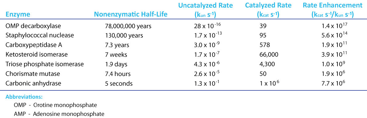
If there is a magical component to life, an argument can surely be made for it being catalysis. Thanks to catalysis, reactions that can take hundreds of years to complete in the uncatalyzed “real world,” occur in seconds in the presence of a catalyst. Chemical catalysts, such as platinum, can speed reactions, but enzymes (which are simply super-catalysts with a “twist,” as we shall see) put chemical catalysts to shame (Figure 4.1). To understand enzymatic catalysis, it is necessary first to understand energy. Chemical reactions follow the universal trend of moving towards lower energy, but they often have a barrier in place that must be overcome. The secret to catalytic action is reducing the magnitude of that barrier.
Before discussing enzymes, it is appropriate to pause and discuss an important concept relating to chemical/biochemical reactions. That concept is equilibrium and it is very often misunderstood. The “equi" part of the word relates to equal, as one might expect, but it does not relate to absolute concentrations. What happens when a biochemical reaction is at equilibrium is that the concentrations of reactants and products do not change over time. This does not mean that the reactions have stopped. Remember that reactions are reversible, so there is a forward reaction and a reverse reaction: if you had 8 molecules of A, and 4 of B at the beginning, and 2 molecules of A were converted to B, while 2 molecules of B were simultaneously converted back to A, the number of molecules of A and B remain unchanged, i.e., the reaction is at equilibrium. However, you will notice that this does not mean that there are equal numbers of A and B molecules.
Concentration Matters
So, contrary to the perceptions of many students, the concentrations of products and reactants are not equal at equilibrium, unless the ΔG°’ for a reaction is zero, because when this is the case,
\[ΔG = \ln \left(\dfrac{[\rm{Products}]}{[\rm{Reactants}]} \right)\]
since the ΔG°’ is zero. Because ΔG itself is zero at equilibrium, then
\[[Products] = [Reactants].\]
This is the only circumstance where
\[[Products] = [Reactants]\]
at equilibrium. Reiterating, at equilibrium, the concentrations of reactant and product do not change over time. That is, for a reaction \(A \rightleftharpoons B [A]\) at time zero when equilibrium is reached, \([A]_{T_0}\), will be the same 5 minutes later (assuming A and B are chemically stable). Thus,
\[[A]_{T_0} = [A]_{T+5}\]
Similarly,
\[[B]_{T_0} = [B]_{T+5}\]
For that matter, at any amount of time X after equilibrium has been reached,
\[[A]T0 = [A]T+5 = [A]TX\]
and
\[[B]T0 = [B] T+5 = [B]TX\]
However, unless ΔG°’ = 0, it is wrong to say [A]T0 = [B]T0 As we study biochemical reactions and reaction rates, it is important to remember that 1) reactions do not generally start at equilibrium; 2) all reactions move in the direction of equilibrium; and 3) reactions in cells behave just like those in test tubes - they do not begin at equilibrium, but they move towards it. Dynamic reactions The reactions occurring in cells, though, are very dynamic and complex. In a test tube, they can be studied one at a time. In cells, the product of one reaction is often the substrate for another one. Reactions in cells are interconnected in this way, giving rise to what are called metabolic pathways. There are, in fact, thousands of different interconnected reactions going on continuously in cells.
Attempts to study a single reaction in the chaos of a cell is daunting to say the least. For this reason, biochemists isolate enzymes from cells and study reactions individually. It is with this in mind that we begin our consideration of the phenomenon of catalysis by describing, first, the way in which enzymes work.
Activation energy
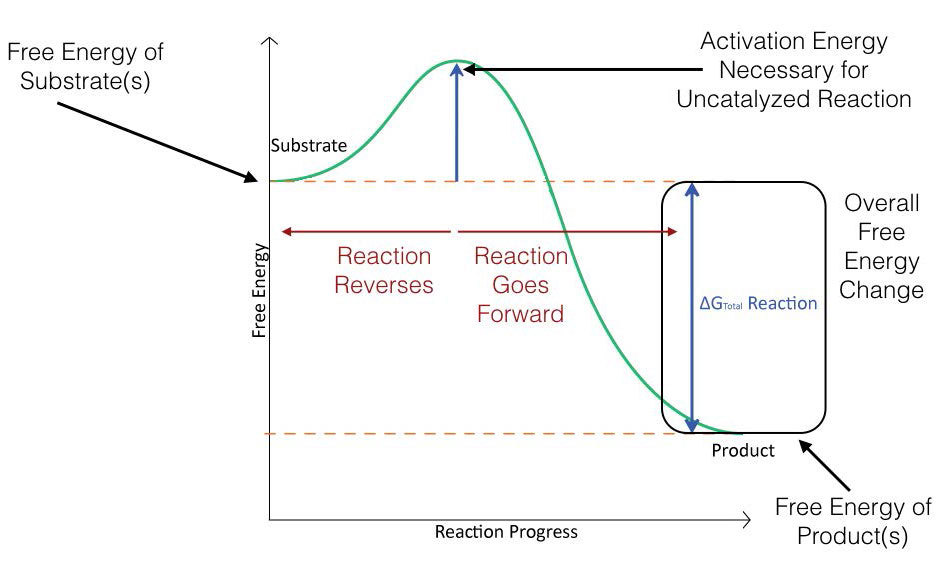
Figure 4.2 schematically depicts the energy changes that occur during the progression of a simple reaction. In order for the reaction to proceed, an activation energy must be overcome in order for the reaction to occur.
In Figure 4.3, the activation energy for a catalyzed reaction is overlaid. As you can see, the reactants start at the same energy level for both catalyzed and uncatalyzed reactions and that the products end at the same energy for both as well. The catalyzed reaction, however, has a lower energy of activation (dotted line) than the uncatalyzed reaction. This is the secret to catalysis - overall ΔG for a reaction does NOT change with catalysis, but the activation energy is lowered.
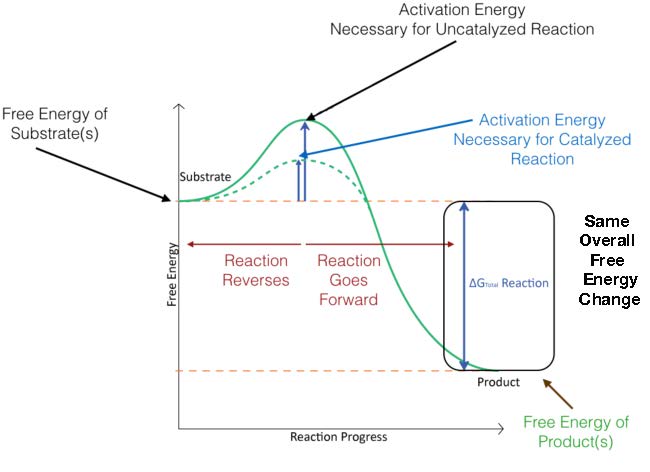
Figure 4.3 - Energy changes during the course of an uncatalyzed reaction (solid green line) and a catalyzed reaction (dotted green line). Image by Aleia Kim
Reversibility
The extent to which reactions will proceed forward is a function of the size of the energy difference between the product and reactant states. The lower the energy of the products compared to the reactants, the larger the percentage of molecules that will be present as products at equilibrium. It is worth noting that since an enzyme lowers the activation energy for a reaction that it can speed the reversal of a reaction just as it speeds a reaction in the forward direction. At equilibrium, of course, no change in concentration of reactants and products occurs. Thus, enzymes speed the time required to reach equilibrium, but do not affect the balance of products and reactants at equilibrium.
Exceptions
The reversibility of enzymatic reactions is an important consideration for equilibrium, the measurement of enzyme kinetics, for Gibbs free energy, for metabolic pathways, and for physiology. There are some minor exceptions to the reversibility of reactions, though. They are related to the disappearance of a substrate or product of a reaction. Consider the first reaction below which is catalyzed by the enzyme carbonic anhydrase:
\[CO_2 + H_2O \rightleftharpoons H_2CO_3 \rightleftharpoons HCO_3^- + H^+\]
In the forward direction, carbonic acid is produced from water and carbon dioxide. It can either remain intact in the solution or ionize to produce bicarbonate ion and a proton. In the reverse direction, water and carbon dioxide are produced. Carbon dioxide, of course, is a gas and can leave the solution and escape.
When reaction molecules are removed, as they would be if carbon dioxide escaped, the reaction is pulled in the direction of the molecule being lost and reversal cannot occur unless the missing molecule is replaced. In the second reaction occurring on the right, carbonic acid (H2CO3) is “removed” by ionization. This too would limit the reaction going back to carbon dioxide in water. This last type of “removal” is what occurs in metabolic pathways. In this case, the product of one reaction (carbonic acid) is the substrate for the next (formation of bicarbonate and a proton).
In the metabolic pathway of glycolysis, ten reactions are connected in this manner and reversing the process is much more complicated than if just one reaction was being considered.
General mechanisms of action
As noted above, enzymatically catalyzed reactions are orders of magnitude faster than uncatalyzed and chemical-catalyzed reactions. The secret of their success lies in a fundamental difference in their mechanisms of action.
Every chemistry student has been taught that a catalyst speeds a reaction without being consumed by it. In other words, the catalyst ends up after a reaction just the way it started so it can catalyze other reactions, as well. Enzymes share this property, but in the middle, during the catalytic action, an enzyme is transiently changed. In fact, it is the ability of an enzyme to change that leads to its incredible efficiency as a catalyst.
Changes
These changes may be subtle electronic ones, more significant covalent modifications, or structural changes arising from the flexibility inherent in enzymes, but not present in chemical catalysts. Flexibility allows movement and movement facilitates alteration of electronic environments necessary for catalysis. Enzymes are, thus, much more efficient than rigid chemical catalysts as a result of their abilities to facilitate the changes necessary to optimize the catalytic process.
Substrate binding
Another important difference between the mechanism of action of an enzyme and a chemical catalyst is that an enzyme has binding sites that not only ‘grab’ the substrate (molecule involved in the reaction being catalyzed), but also place it in a position to be electronically induced to react, either within itself or with another substrate.
The enzyme itself may play a role in the electronic induction or the induction may occur as a result of substrates being placed in very close proximity to each other. Chemical catalysts have no such ability to bind substrates and are dependent upon them colliding in the right orientation at or near their surfaces.
Active site
Reactions in an enzyme are catalyzed at a specific location within it known as the ‘active site’. Substrates bind at the active site and are oriented to provide access for the relevant portion of the molecule to the electronic environment of the enzyme where catalysis occurs.
Enzyme flexibility
As mentioned earlier, a difference between an enzyme and a chemical catalyst is that an enzyme is flexible. Its slight changes in shape (often arising from the binding of the substrate itself) help to optimally position substrates for reaction after they bind.

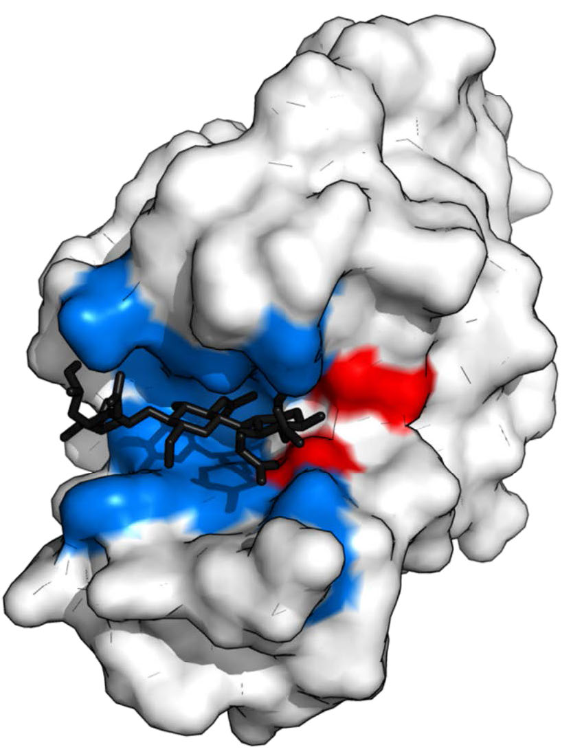
Figure 4.5 - Lysozyme with substrate binding site (blue), active site (red) and bound substrate (black). Wikipedia
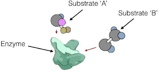
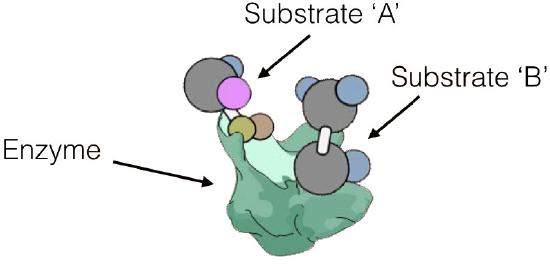
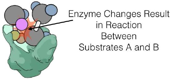
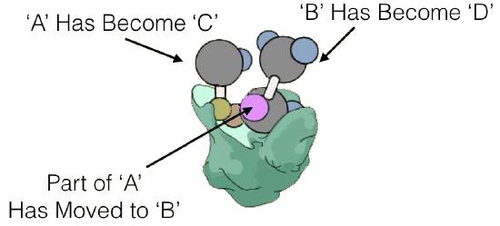
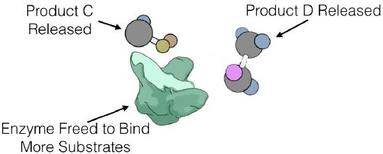
Induced fit
These changes in shape are explained, in part, by Koshland’s Induced Fit Model of Catalysis (Figure 4.6), which illustrates that not only do enzymes change substrates, but that substrates also transiently change enzyme structure. At the end of the catalysis, the enzyme is returned to its original state. Koshland’s model is in contrast to the Fischer Lock and Key model, which says simply that an enzyme has a fixed shape that is perfectly matched for binding its substrate(s). Enzyme flexibility also is important for control of enzyme activity. Enzymes alternate between the T (tight) state, which is a lower activity state and the R (relaxed) state, which has greater activity.

Induced Fit
The Koshland Induced Fit model of catalysis postulates that enzymes are flexible and change shape on binding substrate. Changes in shape help to 1) aid binding of additional substrates in reactions involving more than one substrate and/or 2) facilitate formation of an electronic environment in the enzyme that favors catalysis. This model is in contrast to the Fischer Lock and Key Model of catalysis which considers enzymes as having pre-formed substrate binding sites.
Ordered binding
The Koshland model is consistent with multi-substrate binding enzymes that exhibit ordered binding of substrates. For these systems, binding of the first substrate induces structural changes in the enzyme necessary for binding the second substrate.
There is considerable experimental evidence supporting the Koshland model. Hexokinase, for example, is one of many enzymes known to undergo significant structural alteration after binding of substrate. In this case, the two substrates are brought into very close proximity by the induced fit and catalysis is made possible as a result.
Reaction types
Enzymes that catalyze reactions involving more than one substrate, such as
\[A + B \rightleftharpoons C + D\]
can act in two different ways. Enzymatic reactions can be of several types, as shown in Figure 4.7. In one mechanism, called sequential reactions, at some point in the reaction, both substrates will be bound to the enzyme. There are, in turn, two different ways in which this can occur - random and ordered.
| Types of Reactions | |
|---|---|
| Single Substrate - Single Product | A ⇄ B |
| Single Substrate - Multiple Products | A ⇄ B + C |
| Multiple Substrates - Single Products | A + B ⇄ C |
| Multiple Substrates - Multiple Products | A + B ⇄ C + D |
Consider lactate dehydrogenase, which catalyzes the reaction below:
\[NADH + Pyruvate → Lactate + NAD^+\]
This enzyme requires that NADH must bind prior to the binding of pyruvate. As noted earlier, this is consistent with an induced fit model of catalysis. In this case, binding of the NADH changes the enzyme shape/environment so that pyruvate can bind and without binding of NADH, the substrate cannot access the pyruvate binding site. This type of multiple substrate reaction is called sequential ordered binding, because the binding of substrates must occur in the right order for the reaction to proceed.
Random binding
A second mechanism of binding/catalysis is exhibited by creatine kinase which catalyzes the following reaction:
\[Creatine + ATP → \text{Creatine phosphate} + ADP\]
For this enzyme, substrates can bind to it in any order. Creatine kinase displays sequential random binding. It is worth mentioning that random binding is not inconsistent with Koshland’s induced fit model. Rather, random binding simply means that the enzyme’s induced fit doesn’t affect substrate binding sites and involves other parts of the enzyme. In summary, sequential binding can occur as ordered binding or as random binding.
Double displacement reactions
Not all enzymes that catalyze multi-substrate reactions, though, bind A and B by the sequential mechanisms above. This other category of enzyme includes those that exhibit what are called “ping-pong” (or double displacement) mechanisms. In these enzymes, the enzyme functions as both a catalyst and a carrier of a group between individually bound substrates. Examples of this type of enzyme include the class of enzymes known as transaminases. A general form of the reactions catalyzed by these enzymes is shown in Figure 4.8.
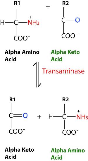
In reversible transaminase reactions, an oxygen and an amine are swapping between the molecules. It can be represented as follows (where N is the amine and O is the oxygen).
A=O + C=N ⇄ B-N + D=O
This reaction occurs not as one transfer reaction swapping the N and the O, but rather as a set of two half-reactions. In this case, the enzyme is a both donor and a carrier of the group being swapped. The first half-reaction goes as follows
A=O + Enz-N ⇄ B-N + Enz=O
Next a second half-reaction goes as
C-N + Enz=O ⇄ D=O + Enz=N
The sum of these half-reactions then is
A=O + C=N ⇄ B-N + D=O
Note that at no time did the enzyme bind both A and C simultaneously. It is also important to recognize that the enzyme existed in two states - Enz=O and Enz-N. The shuffling of the enzyme between these two states is what gives rise to the ping-pong name of this mechanism - it literally goes back and forth like a ping-pong ball in a table tennis match.
Enzyme kinetics
To understand how an enzyme enhances the rate of a reaction, we must understand enzyme kinetics. We present a model here proposed by Leonor Michaelis and Maud Menten. In order to understand the model, it is necessary to understand a few parameters.
First, we describe a reaction in simple terms proceeding as follows
E + S ⇄ ES -> E + P
where E is enzyme, S is substrate, and P is product. In this scheme, ES is the Enzyme-Substrate complex, which is simply the enzyme bound to its substrate.
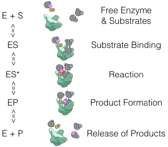
We could define the ES state a bit further with
E + S ⇄ ES -> ES* -> EP -> E + P
where ES* is the activated state and EP is the enzyme-product complex before release of the product.
The first consideration we have is velocity. The velocity of a reaction is the rate of creation of product over time, measured as the concentration of product per time. The time is a critical consideration when measuring velocity. In a closed system (in which an enzyme operates), all reactions will advance towards equilibrium. Enzymatically catalyzed reactions are no different in the end result from non-enzymatic reactions, except that they get to equilibrium faster.
Equilibrium
At equilibrium, the ratio of product to reactant does not change. That is a property of equilibrium. Since the system is closed, the concentration of product over time will not change. The velocity will thus be zero under these conditions and we will have learned nothing about the reaction if we wait too long to study it.
Velocity

Consequently, in Michaelis-Menten kinetics, velocity is measured as initial velocity (V0). This is accomplished by measuring the rate of formation of product early in the reaction before equilibrium is established and under these conditions, there is very little if any of the reverse reaction occurring.
The other two assumptions are related. First, we use conditions where there is much more substrate than enzyme. This makes sense. If the substrate is not in great excess, then the enzyme’s conversion of substrate to product will occur much faster than the enzyme can bind substrate.
Waiting for substrate
Thus, the enzyme would “wait” for substrate to bind if there were not sufficient amounts of it to bind to the enzyme in a timely fashion (when substrate concentration is low). This would not give an accurate measure of velocity, since the enzyme would be inactive a good deal of the time. Because of this, we assume saturation of the enzyme with substrate will give a maximal velocity of the reaction.
Steady state
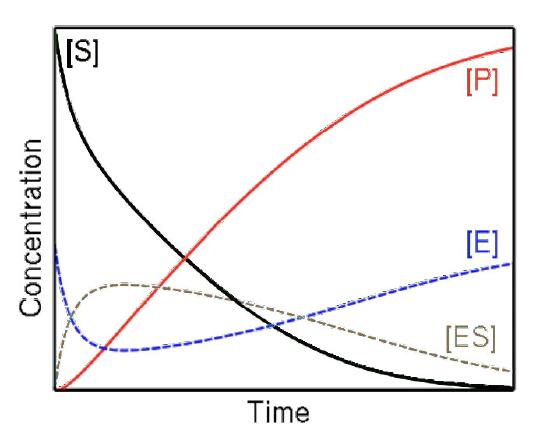
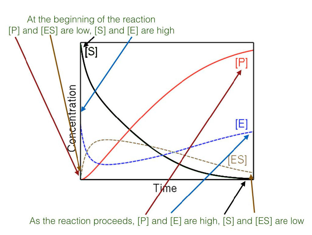
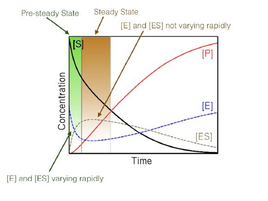
Figure 4.17 - Steady state versus non-steady state conditions
Last, the high concentration of substrate combined with measuring initial conditions results in studying reactions that are under so-called steady state conditions (Figure 4.17). When steady state occurs, the concentration of the ES complex over time is not significantly changing during the period of analysis.
Reiterating, the three assumptions for Michaelis-Menten kinetics are
- Measurement of initial velocity of a reaction
- Substrate in great excess compared to enzyme
- Reaction conditions occurring under steady state
Experimental considerations
Now we turn our attention to how studies of the kinetic properties of an enzyme are conducted. To perform an analysis, one would do the following experiment - 20 different tubes would be set up with enzyme buffer (to keep the enzyme stable), the same amount of enzyme, and then a different amount of substrate in each tube, ranging from tiny amounts in the first tubes to very large amounts in the last tubes. The reaction would be allowed to proceed for a fixed, short amount of time and then the reaction would be stopped and the amount of product contained in each tube would be determined.
The initial velocity (V0) of the reaction then would be the concentration of product found in each tube divided by the time that the reaction was allowed to run. Data from the experiment would be plotted on a graph using initial velocity (V0) on the Y-axis and the concentration of substrate on the X-axis, each tube, of course having a unique reaction velocity corresponding to a unique substrate concentration.
For an enzyme following Michaelis-Menten kinetics, a curve like that shown in Figure 4.18 or 4.19 would result. At low concentration of substrate, it is limiting and the enzyme converts it into product as soon as it can bind it. Consequently, at low concentrations of substrate, the rate of increase of [P] is almost linear with [S] (Figure 4.19).
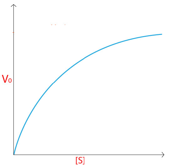
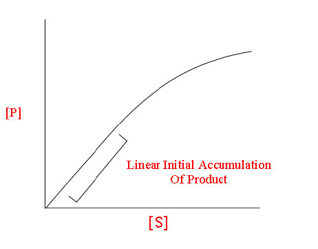
Figure 4.19 - Linear relationship between [P] and [S] at low [S]
Non-linear increase
As the substrate concentration increases, however, the velocity of the reaction in tubes with higher substrate concentration ceases to increase linearly and instead begins to flatten out, indicating that as the substrate concentration gets higher and higher, the enzyme has a harder time keeping up to convert the substrate to product.
Saturation
Not surprisingly, when the enzyme becomes completely saturated with substrate, it will not have to wait for substrate to diffuse to it and will therefore be operating at maximum velocity.
For an enzyme following Michaelis-Menten kinetics will have its velocity (v) at any given substrate concentration given by the following equation:
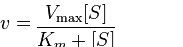
Vmax
Two terms in the equation above require explanation. The first is Vmax. It refers to the maximum velocity of an enzymatic reaction. Maximum velocity for a reaction occurs when an enzyme is saturated with substrate. Saturation is important because it means (per the assumption above) that none of the enzyme molecules are “waiting” for substrate after a product is released. Saturation ensures that another substrate is always instantly available. The unit of Vmax is concentration of product per time = [P]/time.
On a plot of initial velocity versus substrate concentration (V0 vs. [S]), Vmax is the value on the Y axis that the curve asymptotically approaches (dotted line in Figure 4.20). It should be noted that the value of Vmax depends on the amount of enzyme used in a reaction. If you double the amount of enzyme used, you will double the Vmax. If one wanted to compare the velocities of two different enzymes, it would be necessary to use the same amounts of enzyme in the reaction each one catalyzes.
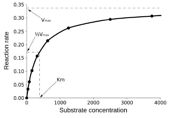
Km
The second term is Km (also known as Ks). Referred to as the Michaelis constant, Km is the substrate concentration that causes the enzyme to work at half of maximum velocity (Vmax/2). What it measures, in simple terms, is the affinity an enzyme has for its substrate. The value of Km is inversely related to the affinity of the enzyme for its substrate. Enzymes with a high Km value will have a lower affinity for their substrate (will take more substrate to get to Vmax/2) whereas those with a low Km will have high affinity and take less substrate to get to Vmax/2. The unit of Km is concentration.
Affinities of enzymes for substrates vary considerably, so knowing Km helps us to understand how well an enzyme is suited to the substrate being used. Measurement of Km depends on the measurement of Vmax.
Common mistake
A common mistake students make in describing Vmax is saying that Km = Vmax /2. This is, of course, not true. Km is a substrate concentration and is the amount of substrate it takes for an enzyme to reach Vmax /2. On the other hand Vmax /2 is a velocity and a velocity certainly cannot equal a concentration.
Kcat
It is desirable to have a measure of velocity that is independent of enzyme concentration. Remember that Vmax depended on the amount of enzyme used. For this, we use the Kcat, also known as the turnover number. Kcat is a number that requires one to first determine Vmax for an enzyme and then divide the Vmax by the concentration of enzyme used to determine Vmax. Thus,
Kcat = Vmax /[Enzyme]
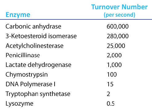
Since Vmax has units of concentration per time and [Enzyme] has units of concentration, the units on Kcat are time-1. While that might seem unintuitive, it means that the value of Kcat is the number of molecules of product made by each molecule of enzyme in the time given. So, a Kcat value of 1000/sec means each enzyme molecule in the reaction at Vmax is producing 1000 molecules of product per second. Note that since Kcat is a calculated value, it cannot be read from a V vs [S] graph as Vmax and Km can.

Amazing Kcat values
A Kcat value of 1000 molecules of product per enzyme per second might seem like a high value, but there are enzymes known (carbonic anhydrase, for example) that have a Kcat value of over 600,000/second (Figure 4.21). This astonishing value illustrates clearly why enzymes seem almost magical in their action. In contrast to \(V_{max}\), which varies with the amount of enzyme used, Kcat is a constant for an enzyme under given conditions.
As seen earlier, enzymes that follow Michaelis-Menten kinetics produce hyperbolic plots of Velocity (V0) versus Substrate Concentration [S] (Figure 4.18). Not all enzymes, though, follow Michaelis-Menten kinetics. Many enzymes have multiple protein subunits and these sometimes interact differently upon binding of a substrate or an external molecule. See ATCase (HERE) for an example.
Perfect enzymes
Now, if we think about what an ideal enzyme might be, it would be one that has a very high velocity and a very high affinity for its substrate. That is, it wouldn’t take much substrate to get to Vmax/2 and the Kcat would be very high. Such enzymes would have values of Kcat / Km that are maximum. Interestingly, there are several enzymes that have this property and their maximal Kcat / Km values are all approximately the same. Such enzymes are referred to as being “perfect” because they have reached the maximum possible value.
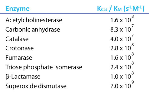
Figure 4.22 - Kcat/Km values for perfect enzymes. Image by Aleia Kim
Diffusion limitation
Why should there be a maximum possible value of Kcat / Km? The answer is that movement of substrate to the enzyme becomes the limiting factor for perfect enzymes. Movement of substrate by diffusion in water has a fixed rate at any temperature and that limitation ultimately determines the maximum speed an enzyme can catalyze at. In a macroscopic world analogy, factories can’t make products faster than suppliers can deliver materials. It is safe to say for a perfect enzyme that the only speed limit it has is the rate of substrate diffusion in water.
Given the “magic” of enzymes alluded to earlier, it might seem that all enzymes should have evolved to be “perfect.” There are very good reasons why most of them have not.
Speed
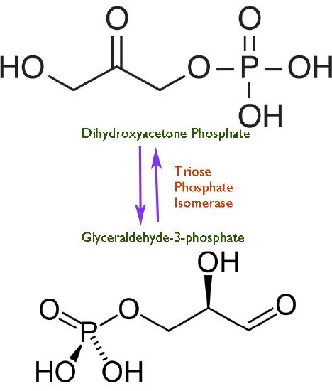
Speed is a dangerous thing. The faster a reaction proceeds in catalysis by an enzyme, the harder it is to control. As we all know from learning to drive, speeding causes accidents. Just as drivers need to have speed limits for operating automobiles, so too must cells exert some control on the ‘throttle’ of their enzymes. In view of this, one might wonder then why any cells have evolved any enzymes to perfection. There is no single answer to the question, but a common one is illustrated by triose phosphate isomerase, which catalyzes a reaction in glycolysis shown in Figure 4.24.
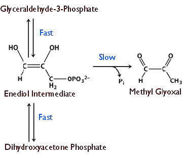
The enzyme appears to have evolved this ability because at lower velocities, there is breakdown of an unstable enediol intermediate that then readily forms methyl glyoxal, a cytotoxic compound (Figure 4.25). Speeding up the reaction provides less opportunity for the unstable intermediate to accumulate and fewer undesirable byproducts to be made.
Dissociation constant
In studying proteins and ligands, it is important to understand the “tightness” with which a protein (P) “holds onto” a ligand (L). This is measured with the dissociation constant (\(K_d\)). The formation of a ligand-protein complex \(LP\) occurs as
\[L + P \rightleftharpoons LP\]
The dissociation of the complex, therefore, is the reverse of this reaction, or
\[LP \rightleftharpoons L + P\]
so the corresponding dissociation constant is defined as
\[K_d = \dfrac{[L][P]}{[LP]}\]
where \([L]\), \([P]\), and \([LP]\) are the molar concentrations of the protein, ligand and the complex when they are joined together.
Smaller values of \(K_d\) indicate tight binding, whereas larger values indicate loose binding. The dissociation constant is the inverse of the association constant.
\[K_a = \dfrac{1}{K_d}\]
Where multiple molecules bond together, such as
\[J_xK_y \rightleftharpoons xJ + yK\]
The complex \(J_xK_y\) is breaking down into \(x\) subunits of \(J\) and \(y\) subunits of \(K\). The dissociation constant is then defined as
\[K_d = \dfrac{[J]^x[K]^y}{[J_xK_y]}\]
where \([J]\), \([K]\), and \([J_xK_y]\) are the concentrations of J, K, and the complex \(J_xK_y\), respectively.
Lineweaver-Burk plots
The study of enzyme kinetics is typically the most math intensive component of biochemistry and one of the most daunting aspects of the subject for many students. Although attempts are made to simplify the mathematical considerations, sometimes they only serve to confuse or frustrate students. Such is the case with modified enzyme plots, such as Lineweaver-Burk (Figure 4.26).
Indeed, when presented by professors as simply another thing to memorize, who can blame students? In reality, both of these plots are aimed at simplifying the determination of parameters, such as \(K_m\) and \(V_{max}\). In making either of these modified plots, it is important to recognize that the same data is used as in making a V0 vs. [S] plot. The data are simply manipulated to make the plotting easier.
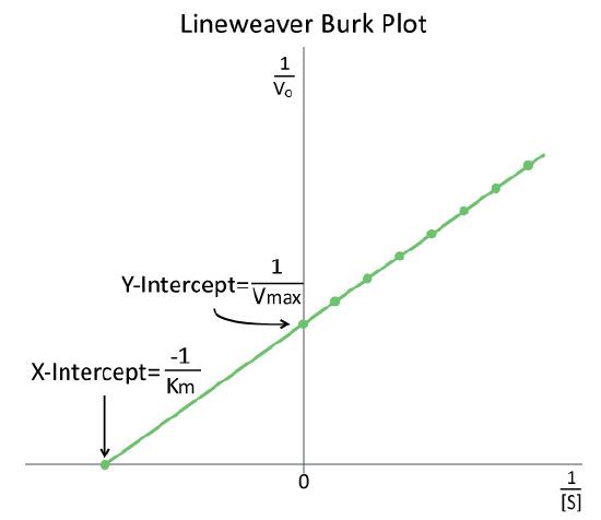
Figure 4.26 - A Lineweaver-Burk plot of \(1/V_0\) vs \(1/[S]\). Image by Aleia Kim
Double reciprocal
For a LineWeaver-Burk plot, the manipulation is using the reciprocal of the values of both the velocity and the substrate concentration. The inverted values are then plotted on a graph as 1/V0 vs. 1/[S]. Because of these inversions, Lineweaver-Burk plots are commonly referred to as ‘double-reciprocal’ plots. As can be seen in Figure 4.26, the value of Km on a Lineweaver Burk plot is easily determined as the negative reciprocal of the x-intercept , whereas the Vmax is the inverse of the y-intercept. Other related manipulation of kinetic data include Eadie-Hofstee diagrams, which plots V0 vs V0/[S] and gives Vmax as the Y-axis intercept with the slope of the line being -Km.
Molecularity of reactions
The term molecularity refers to the number of molecules that must come together in order for a reaction to take place. Reactions of the sort of A -> B (where ‘A’ is the reactant and ‘B’ is the product) are unimolecular, since A is directly changed into B. The rate of the reaction is related only to the concentration of reactant A. For a bimolecular reaction where A + B ⇄ C the reaction depends on the concentration of both A and B and its rate will be related to the product of the concentration of A and of B.
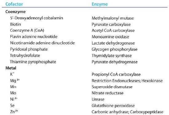
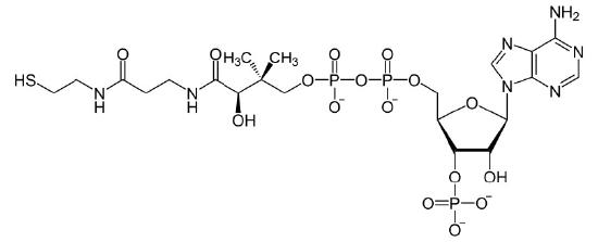
Coenzymes
Organic molecules that assist enzymes and facilitate catalysis are co-factors called coenzymes. The term co-factor is a broad category usually subdivided into inorganic ions and coenzymes. If the coenzyme is very tightly or covalently bound to the enzyme, it is referred to as a prosthetic group. Enzymes without their co-factors are inactive and referred to as apoenzymes. Enzymes containing all of their co-factors are called holoenzymes.
Pre-steady state kinetic studies
In the study of kinetic rates of enzymatic reactions, time zero is a very critical point. It establishes when the mixing of substrate with enzyme and measurement of formation of product begins. At time zero, there is no product. As shown in Figure 4.29, the appearance of product (on a short time scale) goes through an early burst phase with a steep slope for [product]/time and then changes.
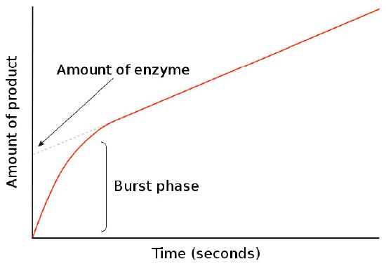
Figure 4.29 - Burst phase of product formation
This change occurs during a critical period in an enzymatic reaction and gives information about the rate of reaction cycles. The duration of the burst phase tells how long a single reaction turnover occurs, whereas the slow of the line post-burst phase tells the amount of “functional” enzyme performing the reaction.
After the burst phase, the slope of the line of the amount of product versus time decreases. This is due to the reaction entering conditions of steady state, used to study Michaelis-Menten kinetics. In steady state conditions, the amount of the enzyme-substrate complex (ES) is relatively constant over time. In simple terms, this occurs when the rate of formation of the ES complex equals the rate of conversion of the substrate to product by the enzyme with release of the product.
Earlier events
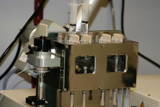
Events occurring prior to the conditions of steady state are referred to as pre-steady state. Depending on the enzyme, in as short as a few milliseconds, steady state conditions can be present meaning that if one hopes to study formation of reaction intermediates in pre-steady state, tools for this analysis must work very rapidly. One instrument commonly used for studying pre-steady state kinetics is called a stopped flow instrument.
It loads an enzyme solution and a substrate into separate syringes whose output is pointed into a mixing chamber. The solutions are rapidly mixed and measurements of product concentration begin. With a stopped flow instrument, dead times (time between mixing and detection) can be achieved of as small as 0.3 msec.
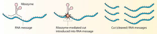
Ribozymes
Proteins do not have a monopoly on acting as biological catalysts. Some RNA molecules are also capable of speeding reactions. The most famous of these molecules was discovered by Tom Cech in the early 1980s Studying excision of an intron in Tetrahymena, Cech was puzzled at his inability to find any proteins catalyzing the process. Ultimately, the catalysis was recognized as coming from the intron itself. It was a self-splicing RNA and since then, many other examples of catalytic RNAs have been found. Catalytic RNA molecules are known as ribozymes.
 359
359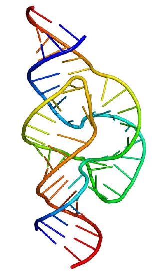
Not unusual
Ribozymes, however, are not rarities of nature. The protein-making ribosomes of cells are essentially giant ribozymes. The 23S rRNA of the prokaryotic ribosome and the 28S rRNA of the eukaryotic ribosome catalyze the formation of peptide bonds.
Ribozymes are also important in our understanding of the evolution of life on Earth. They have been shown to be capable via selection to evolve self-replication. Indeed, ribozymes actually answer a chicken/egg dilemma - which came first, enzymes that do the work of the cell or nucleic acids that carry the information required to produce the enzymes. As both carriers of genetic information and catalysts, ribozymes are likely both the chicken and the egg in the origin of life.